6. Contrôle de trajectoires

Marc BUFFAT, dpt mécanique, Université Claude Bernard Lyon 1

Mise à disposition selon les termes de la Licence Creative Commons Attribution - Pas d’Utilisation Commerciale - Partage dans les Mêmes Conditions 2.0 France

%matplotlib inline
import numpy as np
import sympy as sp
import matplotlib.pyplot as plt
from IPython.core.display import HTML
from IPython.display import display,Image
from sympy.physics.vector import init_vprinting
init_vprinting(use_latex='mathjax', pretty_print=False)
plt.rc('font', family='serif', size='14')

6.1. Problème: pont roulant

6.1.1. objectif

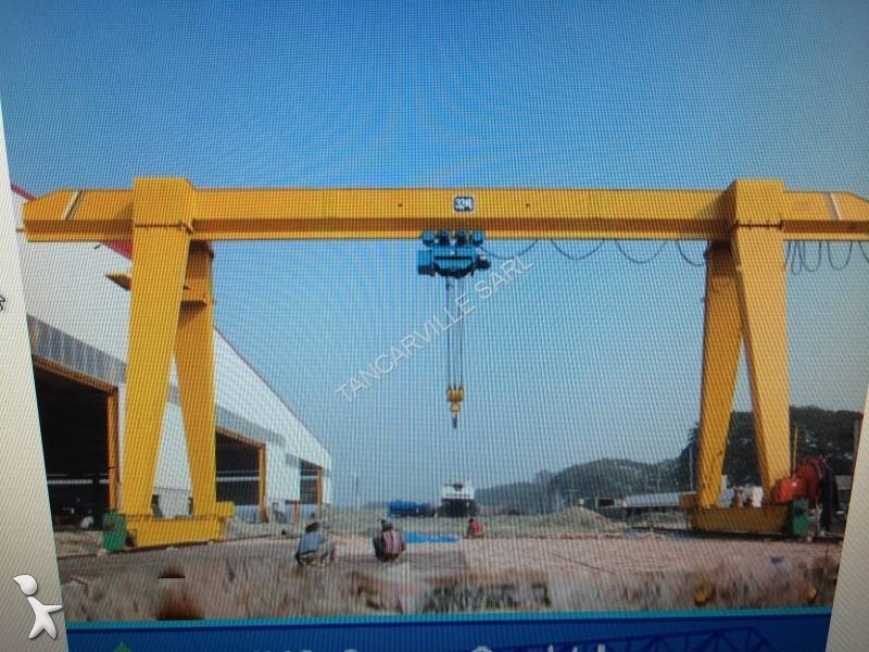
On veut déplacer, à l’aide d’un système de levage par câble (grue ou pont roulant), une charge d’un endroit à un autre en évitant les oscillations résiduelles à l’arrivée. L’objectif est de proposer une stratégie de commande simple et réaliste qui repose sur une structure de commande hiérarchisée, composée de régulateurs de bas niveau rapides, simples et découplés et d’une commande de haut niveau lente et prenant en compte les couplages. En outre, on mesure la position et la vitesse du chariot ainsi que la position et la vitesse du treuil, mais la position de la charge n’est pas mesurée. C’est pourquoi nous ne considérons que des bouclages qui ne dépendent que des positions et vitesses du chariot et du treuil.

6.1.2. modélisation

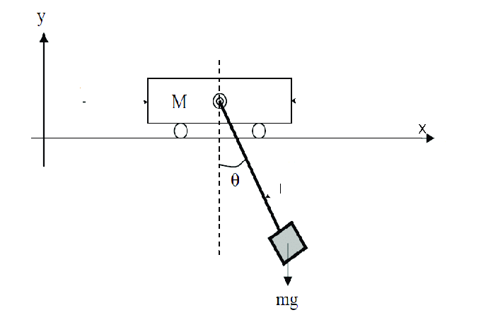
• modèle mécanique;

pendule P de masse m de longueur \(l(t)\) accroché à un chariot C de masse M se deplacant horizontalement \(x_c(t)\)

• système à 3 ddl \(xc(t), \theta(t), l(t) \)

6.1.3. repère et ddl

from sympy.physics.mechanics import dynamicsymbols, Point, ReferenceFrame
from sympy.physics.mechanics import Particle, RigidBody, Lagrangian, LagrangesMethod

# parametres
theta,  xc, l    = dynamicsymbols("theta x_c l")
thetap, xcp, lp = dynamicsymbols("theta x_c l",1)
m,M,g  = sp.symbols('m M g')
t      = sp.Symbol('t')

# pt et répère
O  = Point('O')
RO = ReferenceFrame("R_O")
C  = Point('C')
C.set_pos(O,xc*RO.x)
RP = ReferenceFrame("R_P")
RP.orient(RO,"Axis",[theta,RO.z])
P = Point('P')
P.set_pos(C, -l*RP.y)
display(C.pos_from(O))
display(P.pos_from(O))

\[\displaystyle x_{c}\mathbf{\hat{r_o}_x}\]

\[\displaystyle - l\mathbf{\hat{r_p}_y} + x_{c}\mathbf{\hat{r_o}_x}\]

6.1.4. cinématique

O.set_vel(RO,0.)
C.set_vel(RO,xcp*RO.x)
P.set_vel(RP, -lp*RP.y)
display(C.vel(RO))
display(P.vel(RP))
P.v1pt_theory(C,RO,RP)

\[\displaystyle \dot{x}_{c}\mathbf{\hat{r_o}_x}\]

\[\displaystyle - \dot{l}\mathbf{\hat{r_p}_y}\]

\[\displaystyle l \dot{\theta}\mathbf{\hat{r_p}_x} - \dot{l}\mathbf{\hat{r_p}_y} + \dot{x}_{c}\mathbf{\hat{r_o}_x}\]

Pc = Particle('P_c',C,M)
Pa = Particle('P_a',P,m)
display(Pa.kinetic_energy(RO))
Pa.potential_energy = m*g*Pa.point.pos_from(C).dot(RO.y)
display(Pa.potential_energy)

\[\displaystyle \frac{m \left(l \cos{\left(\theta \right)} \dot{\theta} + \sin{\left(\theta \right)} \dot{l}\right) \dot{x}_{c}}{2} + \frac{m l^{2} \dot{\theta}^{2}}{2} + \frac{m l \cos{\left(\theta \right)} \dot{\theta} \dot{x}_{c}}{2} + \frac{m \sin{\left(\theta \right)} \dot{l} \dot{x}_{c}}{2} + \frac{m \dot{l}^{2}}{2} + \frac{m \dot{x}_{c}^{2}}{2}\]

\[\displaystyle - g m l \cos{\left(\theta \right)}\]

6.1.5. Lagrangien

La = Lagrangian(RO,Pa,Pc)
display(La)

\[\displaystyle \frac{M \dot{x}_{c}^{2}}{2} + g m l \cos{\left(\theta \right)} + \frac{m \left(l \cos{\left(\theta \right)} \dot{\theta} + \sin{\left(\theta \right)} \dot{l}\right) \dot{x}_{c}}{2} + \frac{m l^{2} \dot{\theta}^{2}}{2} + \frac{m l \cos{\left(\theta \right)} \dot{\theta} \dot{x}_{c}}{2} + \frac{m \sin{\left(\theta \right)} \dot{l} \dot{x}_{c}}{2} + \frac{m \dot{l}^{2}}{2} + \frac{m \dot{x}_{c}^{2}}{2}\]

6.1.6. Bilan des forces

• force motrice \(F_c\) sur le chariot en C

• force de tension \(T\) dans le cable (ne travaille pas)

• couple sur un treuil de rayon \(\rho\)

  • rayon \(\rho\) (on néglige son inertie \(J_\rho\))

  • angle \(\phi = (l-l_0)/\rho\)

  • couple \(C_t\)

  • travail \(C_t \rho \delta l \)

Fc, Ct, rho, l0 = sp.symbols('F_c C_t rho l_0')
phi_t = (l-l0)/rho
Rt  = ReferenceFrame('R_t')
Rt.orient(RO,'Axis',[phi_t,RO.z])

display(La)
LM = LagrangesMethod(La,[theta,xc,l],forcelist=[(C,Fc*RO.x),(Rt,-Ct*m*rho*RO.z)], frame = RO)
eq = sp.simplify(LM.form_lagranges_equations())
display(eq)

\[\displaystyle \frac{M \dot{x}_{c}^{2}}{2} + g m l \cos{\left(\theta \right)} + \frac{m \left(l \cos{\left(\theta \right)} \dot{\theta} + \sin{\left(\theta \right)} \dot{l}\right) \dot{x}_{c}}{2} + \frac{m l^{2} \dot{\theta}^{2}}{2} + \frac{m l \cos{\left(\theta \right)} \dot{\theta} \dot{x}_{c}}{2} + \frac{m \sin{\left(\theta \right)} \dot{l} \dot{x}_{c}}{2} + \frac{m \dot{l}^{2}}{2} + \frac{m \dot{x}_{c}^{2}}{2}\]

\[\begin{split}\displaystyle \left[\begin{matrix}m \left(g \sin{\left(\theta \right)} + l \ddot{\theta} + \cos{\left(\theta \right)} \ddot{x}_{c} + 2 \dot{l} \dot{\theta}\right) l\\- F_{c} + M \ddot{x}_{c} - m l \sin{\left(\theta \right)} \dot{\theta}^{2} + m l \cos{\left(\theta \right)} \ddot{\theta} + m \sin{\left(\theta \right)} \ddot{l} + 2 m \cos{\left(\theta \right)} \dot{l} \dot{\theta} + m \ddot{x}_{c}\\m \left(C_{t} - g \cos{\left(\theta \right)} - l \dot{\theta}^{2} + \sin{\left(\theta \right)} \ddot{x}_{c} + \ddot{l}\right)\end{matrix}\right]\end{split}\]

6.2. Chariot immobile

• \(\dot{x_c}=0\)

• la force de tension ne travaille pas (liaison parfaite)

• mouvement \(l(t)\) imposé

LLa = sp.simplify(La.subs({xcp:0}))
display(LLa)

\[\displaystyle \frac{m \left(2 g l \cos{\left(\theta \right)} + l^{2} \dot{\theta}^{2} + \dot{l}^{2}\right)}{2}\]

LM = LagrangesMethod(LLa,[theta])
eq=sp.simplify(LM.form_lagranges_equations()[0]/(m*l))
display(eq)

\[\displaystyle g \sin{\left(\theta \right)} + l \ddot{\theta} + 2 \dot{l} \dot{\theta}\]

6.2.1. interprétation

• variation moment cinétique suivant Ro.y = moment poids

pz = Pa.angular_momentum(C,RO).subs({xcp:0}).dot(RO.z)
display(pz)
pz.diff(t) + -m*g*(RO.y.cross(P.pos_from(C)).dot(RO.z))

\[\displaystyle m l^{2} \dot{\theta}\]

\[\displaystyle g m l \sin{\left(\theta \right)} + m l^{2} \ddot{\theta} + 2 m l \dot{l} \dot{\theta}\]

6.2.2. linéarisation

• \(l \approx l_0\)

• \(\dot{l} = \omega l_0\)

• solution amortie ou amplifiée

l0 , omega = sp.symbols('l_0 omega')
eq0=sp.simplify(eq.subs({lp:omega*l0,l:l0,g:omega**2*l0,sp.sin(theta):theta})/l0)
display(eq0)

\[\displaystyle \omega^{2} \theta + 2 \omega \dot{\theta} + \ddot{\theta}\]

theta0 = sp.Symbol('theta_0')
sol = sp.dsolve(eq0,ics={theta.subs(t,0):theta0, theta.diff(t).subs(t,0):0})
display(sol)

\[\displaystyle \theta = \left(\omega t \theta_{0} + \theta_{0}\right) e^{- \omega t}\]

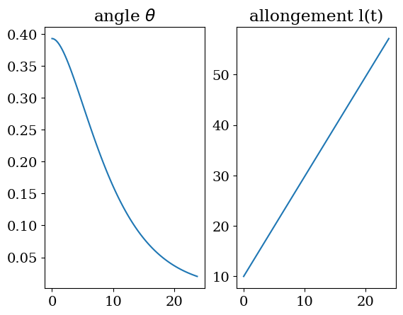
6.2.3. simulation cas linéarisé

Theta=sp.lambdify([t,theta0,omega],sol.rhs,'numpy')

L0     = 10.0
GG     = 9.81
OMEGA0 = 0.2*np.sqrt(GG/L0)
THETA0 = np.pi/8
TF     = 1.5*np.pi/OMEGA0
tt    = np.linspace(0,TF,100)
THETA = Theta(tt,THETA0,OMEGA0)
LL    = L0+OMEGA0*L0*tt

plt.subplot(1,2,1)
plt.plot(tt,THETA)
plt.title('angle $\\theta$')
plt.subplot(1,2,2)
plt.plot(tt,LL)
plt.title("allongement l(t)")

Text(0.5, 1.0, 'allongement l(t)')

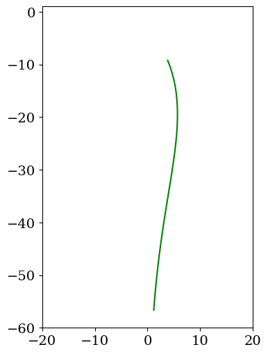
6.2.4. animation cas linéaire

from validation.Chariot import Pendule,Chariot

pas = 2
pendule = Pendule(LL[0::pas],THETA[0::pas],tt[pas])
anim = pendule.calculanim(-20,20,-60,1);

plt.rc('animation', html='jshtml')
anim

Once Loop Reflect

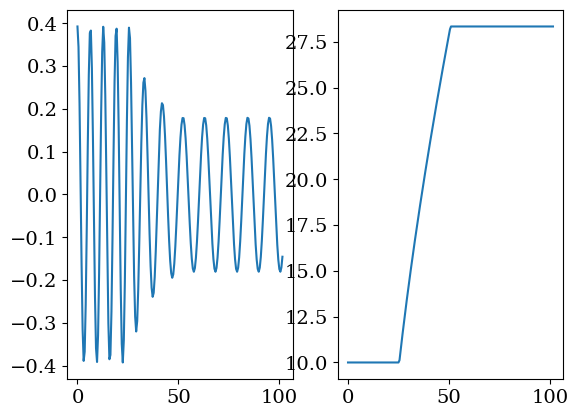
6.2.5. simulation cas non linéaire

• resolution \(Y = [\theta, \dot\theta, l]\)

• equation sur \(l\)

  • si \(t > T_1\) $\(\frac{dl}{dt} = 0 \)$

  • si \(t > T_1\) et \(t<2 T_1\) $\(\frac{dl}{dt} = \sqrt{\frac{g}{l}} \)$

  • sinon $\(\frac{dl}{dt} = 0 \)$

6.2.6. equations de Lagrange à l’ordre 1

\[ \dot{Y} = F(Y,t) \]

smb = sp.simplify(LM.rhs())
display(smb)
smbF = sp.lambdify([theta,thetap,l,lp,g],smb,'numpy')

\[\begin{split}\displaystyle \left[\begin{matrix}\dot{\theta}\\- \frac{g \sin{\left(\theta \right)} + 2 \dot{l} \dot{\theta}}{l}\end{matrix}\right]\end{split}\]

6.2.7. simulation numérique

# parametres
OMEGA0 = np.sqrt(GG/L0)
T1 = 4*2*np.pi/OMEGA0
def F(Y,t):
    global L0
    Lp = 0.0
    if (t>T1) and (t<2*T1): Lp = np.sqrt(GG/Y[2])
    FF = smbF(Y[0],Y[1],Y[2],Lp,GG)
    dY = np.array([FF[0,0],FF[1,0],Lp])
    return dY

from scipy.integrate import odeint
Y0 = [THETA0,0.,L0]
TT = 4*T1
tt  = np.linspace(0,TT,200)
sol = odeint(F,Y0,tt)
THETA = sol[:,0]
LL    = sol[:,2]

plt.subplot(1,2,1)
plt.plot(tt,THETA)
plt.subplot(1,2,2)
plt.plot(tt,LL)

[<matplotlib.lines.Line2D at 0x7fe896eec700>]

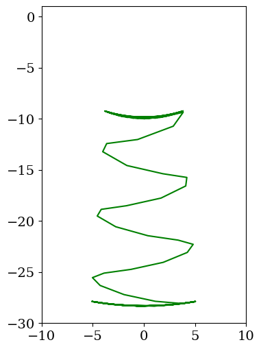
6.2.8. animation

pas = 2
pendule = Pendule(LL[0::pas],THETA[0::pas],tt[pas])
anim = pendule.calculanim(-10,10,-30,1);

plt.rc('animation', html='jshtml')
anim

Once Loop Reflect

6.2.9. Conclusion

on ne contrôle pas le mouvement de la charge !!

6.3. Chariot mobile, longueur fixe

• on applique une force horizontale \(F_c\) avec un cable de longueur \(l_0\)

• adim: \( F_c M = F_c \alpha m \)

• \(\alpha = \frac{M}{m}\)

• objectif:

  • déterminer la force \(F_c\) pour avoir un ballant minimum

  • tests de différents contrôle

    • contrôle du chariot seule

    • asservissement de la trajectoire du chariot

    • couplage de haut niveau

alpha = sp.Symbol('alpha')
LLa = sp.simplify(La.subs({lp:0,l:l0,M:alpha*m}))
display(LLa)

\[\displaystyle \frac{m \left(\alpha \dot{x}_{c}^{2} + 2 g l_{0} \cos{\left(\theta \right)} + l_{0}^{2} \dot{\theta}^{2} + 2 l_{0} \cos{\left(\theta \right)} \dot{\theta} \dot{x}_{c} + \dot{x}_{c}^{2}\right)}{2}\]

6.3.1. equations de Lagrange

Fc = sp.symbols('F_c')
LM = LagrangesMethod(LLa,[theta,xc],forcelist=[(C,Fc*alpha*m*RO.x)], frame = RO)
eq = sp.simplify(LM.form_lagranges_equations())
display(eq)

\[\begin{split}\displaystyle \left[\begin{matrix}l_{0} m \left(g \sin{\left(\theta \right)} + l_{0} \ddot{\theta} + \cos{\left(\theta \right)} \ddot{x}_{c}\right)\\m \left(- F_{c} \alpha + \alpha \ddot{x}_{c} - l_{0} \sin{\left(\theta \right)} \dot{\theta}^{2} + l_{0} \cos{\left(\theta \right)} \ddot{\theta} + \ddot{x}_{c}\right)\end{matrix}\right]\end{split}\]

display(LM.mass_matrix)
display(sp.simplify(LM.forcing))

\[\begin{split}\displaystyle \left[\begin{matrix}l_{0}^{2} m & l_{0} m \cos{\left(\theta \right)}\\l_{0} m \cos{\left(\theta \right)} & \frac{m \left(2 \alpha + 2\right)}{2}\end{matrix}\right]\end{split}\]

\[\begin{split}\displaystyle \left[\begin{matrix}- g l_{0} m \sin{\left(\theta \right)}\\m \left(F_{c} \alpha + l_{0} \sin{\left(\theta \right)} \dot{\theta}^{2}\right)\end{matrix}\right]\end{split}\]

display(sp.simplify(LM.rhs()).doit())

\[\begin{split}\displaystyle \left[\begin{matrix}\dot{\theta}\\\dot{x}_{c}\\- \frac{F_{c} \alpha \cos{\left(\theta \right)} + \alpha g \sin{\left(\theta \right)} + g \sin{\left(\theta \right)} + \frac{l_{0} \sin{\left(2 \theta \right)} \dot{\theta}^{2}}{2}}{l_{0} \left(\alpha + \sin^{2}{\left(\theta \right)}\right)}\\\frac{F_{c} \alpha + \frac{g \sin{\left(2 \theta \right)}}{2} + l_{0} \sin{\left(\theta \right)} \dot{\theta}^{2}}{\alpha + \sin^{2}{\left(\theta \right)}}\end{matrix}\right]\end{split}\]

6.3.2. Contrôle simple du chariot

On contrôle uniquement le chariot \(x_c(t)\)

\[ (1+\alpha)\ddot{x_c} = \alpha F_c\]

• on impose une trajectoire au chariot tq. $\( x_c(0)=0, \dot{x_c}(0)=0, x_c(t_f) = x_f, \dot{x_c}(t_f)=0\)$

• \(x_c(t)\) polynôme de degré 3

\[ x_c(t) = x_f \frac{t^2}{t_f^2}(3-2\frac{t}{t_f})\]

• d’où la force \(F_c\) sur le chariot

xf,tf = sp.symbols('x_f t_f')
xcc = xf*t**2*(3*tf-2*t)/tf**3
display(xcc)
xcc.diff(t).subs(t,tf)

\[\displaystyle \frac{t^{2} x_{f} \left(- 2 t + 3 t_{f}\right)}{t_{f}^{3}}\]

\[\displaystyle 0\]

Fcc = (1+alpha)/alpha*xcc.diff(t,2)
display(Fcc)

\[\displaystyle - \frac{2 x_{f} \left(\alpha + 1\right) \left(6 t - 3 t_{f}\right)}{\alpha t_{f}^{3}}\]

# force sur le chariot
FCX = sp.lambdify([t,tf,xf,alpha],Fcc,'numpy')

6.3.3. Asservissement simple

• on applique un asservissement simple pour avoir la trajectoire précédente

\[ x_i(t) = x_f \frac{t^2}{t_f^2}(3-2\frac{t}{t_f})\]

• asservissement $\( F_a(t) = -K_c \left( (x(t)-x_i(t)) + T_c(\dot x - \dot x_i) \right) \)$

Kc,Tc = sp.symbols('K_c T_c')
Fca = -Kc*((xc-xcc)+Tc*(xcp-xcc.diff(t)))
display(Fca)

\[\displaystyle - K_{c} \left(T_{c} \left(\frac{2 t^{2} x_{f}}{t_{f}^{3}} - \frac{2 t x_{f} \left(- 2 t + 3 t_{f}\right)}{t_{f}^{3}} + \dot{x}_{c}\right) - \frac{t^{2} x_{f} \left(- 2 t + 3 t_{f}\right)}{t_{f}^{3}} + x_{c}\right)\]

# force sur le treuil
FCA = sp.lambdify([t,tf,xf,xc,xcp,Kc,Tc],Fca,'numpy')

6.3.4. Commande de haut niveau lente

• linéarisation des équations

• controle du positionnement de la charge

6.3.4.1. mouvement de la charge

• coordonnees \(\xi(t)\), \(\eta(t)\) dans le repere fixe

display(P.pos_from(O).express(RO))
xi, eta = dynamicsymbols('xi eta')
display(sp.Eq(xi,P.pos_from(O).dot(RO.x)))
display(sp.Eq(eta,P.pos_from(O).dot(RO.y)))
display(sp.Eq(sp.tan(theta),(-xi+xc)/eta))

\[\displaystyle (l \sin{\left(\theta \right)} + x_{c})\mathbf{\hat{r_o}_x} - l \cos{\left(\theta \right)}\mathbf{\hat{r_o}_y}\]

\[\displaystyle \xi = l \sin{\left(\theta \right)} + x_{c}\]

\[\displaystyle \eta = - l \cos{\left(\theta \right)}\]

\[\displaystyle \tan{\left(\theta \right)} = \frac{x_{c} - \xi}{\eta}\]

6.3.4.2. parametrisation / trajectoire

• equation d’équilibre de la charge en fonction de la tension T

T = sp.Symbol('T')
display(sp.Eq(m*xi.diff(t,t) , -T*sp.sin(theta)))
display(sp.Eq(m*eta.diff(t,t),  T*sp.cos(theta) - m*g))
display(sp.Eq(sp.tan(theta), -xi.diff(t,t)/(eta.diff(t,t)+g)))
display(sp.Eq(xc, xi - eta*xi.diff(t,t)/(eta.diff(t,t)+g)) )

\[\displaystyle m \ddot{\xi} = - T \sin{\left(\theta \right)}\]

\[\displaystyle m \ddot{\eta} = T \cos{\left(\theta \right)} - g m\]

\[\displaystyle \tan{\left(\theta \right)} = - \frac{\ddot{\xi}}{g + \ddot{\eta}}\]

\[\displaystyle x_{c} = \xi - \frac{\eta \ddot{\xi}}{g + \ddot{\eta}}\]

6.3.4.3. paramétrisation

si on connait \(xi(t)\) et \(eta(t)\) jusqu’à leurs dérivées d’ordre 4, peut donc déterminer le mouvement et calculer la force \(F_c\)

6.3.4.4. linéarisation \(\theta\) petit

• \(\eta = - l_0\)

• \(\theta = -\frac{\ddot{\xi}}{g}\)

• \(x_c = \xi + \frac{l_0}{g} \ddot{\xi}\)

• \(\omega_0 ^2 = \frac{g}{l_0}\)

calcul de la force \(F_c\)

omega0 = sp.Symbol('omega_0')
eq0=sp.simplify(eq[1].subs({sp.cos(theta):1,sp.sin(theta):0})/m)
display(eq0)
eq1=eq0.subs({xc.diff(t,2):xi.diff(t,2)+l0/g*xi.diff(t,4),theta.diff(t,2):-xi.diff(t,4)/g, g: omega0**2*l0})
display(eq1)
Fc1=(alpha*Fc+eq1)/alpha
display(sp.Eq(Fc,Fc1))

\[\displaystyle - F_{c} \alpha + \alpha \ddot{x}_{c} + l_{0} \ddot{\theta} + \ddot{x}_{c}\]

\[\displaystyle - F_{c} \alpha + \alpha \left(\ddot{\xi} + \frac{\ddddot{\xi}}{\omega_{0}^{2}}\right) + \ddot{\xi}\]

\[\displaystyle F_{c} = \frac{\alpha \left(\ddot{\xi} + \frac{\ddddot{\xi}}{\omega_{0}^{2}}\right) + \ddot{\xi}}{\alpha}\]

6.3.4.5. trajectoire

• trajectoire \(\xi(t)\) tq. $\(\xi(0)=0, \frac{d\xi}{dt}(0)=0, \frac{d^2\xi}{dt^2}(0)=0, \frac{d^3\xi}{dt^3}(0)=0, \frac{d^4\xi}{dt^4}(0)=0\)\( \)\(\xi(t_f)=x_f, \frac{d\xi}{dt}(t_f)=0, \frac{d^2\xi}{dt^2}(t_f)=0, \frac{d^3\xi}{dt^3}(t_f)=0, \frac{d^4\xi}{dt^4}(t_f)=0\)$

• \(\xi(t)\) polynome de degré 9 en t

xf, tf = sp.symbols('x_f t_f')
x = xf*(t/tf)**5*(126-420*(t/tf)+540*(t/tf)**2-315*(t/tf)**3+70*(t/tf)**4)
display(sp.Eq(xi,x))
# verification
print("dérivées en tf:",x.diff(t,1).subs({t:tf}),x.diff(t,2).subs({t:tf}),x.diff(t,3).subs({t:tf}),x.diff(t,4).subs({t:tf}))
# contrôle Fc
Fcx=Fc1.subs({xi.diff(t,4):x.diff(t,4),xi.diff(t,2):x.diff(t,2)}).doit().simplify()
display(sp.Eq(Fc,Fcx))
# position chariot xc
xcx= xi + xi.diff(t,2)/omega0**2
xcx= xcx.subs({xi:x}).doit().simplify()
display(sp.Eq(xc,xcx))
# angle theta
thx= -xi.diff(t,2)/(l0*omega0**2)
thx= thx.subs({xi:x}).doit().simplify()
display(sp.Eq(theta,thx))

\[\displaystyle \xi = \frac{t^{5} x_{f} \left(\frac{70 t^{4}}{t_{f}^{4}} - \frac{315 t^{3}}{t_{f}^{3}} + \frac{540 t^{2}}{t_{f}^{2}} - \frac{420 t}{t_{f}} + 126\right)}{t_{f}^{5}}\]

dérivées en tf: 0 0 0 0

\[\displaystyle F_{c} = \frac{2520 t x_{f} \left(2 \alpha \omega_{0}^{2} t^{6} - 7 \alpha \omega_{0}^{2} t^{5} t_{f} + 9 \alpha \omega_{0}^{2} t^{4} t_{f}^{2} - 5 \alpha \omega_{0}^{2} t^{3} t_{f}^{3} + \alpha \omega_{0}^{2} t^{2} t_{f}^{4} + 84 \alpha t^{4} - 210 \alpha t^{3} t_{f} + 180 \alpha t^{2} t_{f}^{2} - 60 \alpha t t_{f}^{3} + 6 \alpha t_{f}^{4} + 2 \omega_{0}^{2} t^{6} - 7 \omega_{0}^{2} t^{5} t_{f} + 9 \omega_{0}^{2} t^{4} t_{f}^{2} - 5 \omega_{0}^{2} t^{3} t_{f}^{3} + \omega_{0}^{2} t^{2} t_{f}^{4}\right)}{\alpha \omega_{0}^{2} t_{f}^{9}}\]

\[\displaystyle x_{c} = \frac{t^{3} x_{f} \left(70 \omega_{0}^{2} t^{6} - 315 \omega_{0}^{2} t^{5} t_{f} + 540 \omega_{0}^{2} t^{4} t_{f}^{2} - 420 \omega_{0}^{2} t^{3} t_{f}^{3} + 126 \omega_{0}^{2} t^{2} t_{f}^{4} + 5040 t^{4} - 17640 t^{3} t_{f} + 22680 t^{2} t_{f}^{2} - 12600 t t_{f}^{3} + 2520 t_{f}^{4}\right)}{\omega_{0}^{2} t_{f}^{9}}\]

\[\displaystyle \theta = \frac{2520 t^{3} x_{f} \left(- 2 t^{4} + 7 t^{3} t_{f} - 9 t^{2} t_{f}^{2} + 5 t t_{f}^{3} - t_{f}^{4}\right)}{l_{0} \omega_{0}^{2} t_{f}^{9}}\]

# fonctions numériques
XI = sp.lambdify([t,xf,tf],x,'numpy')
XC = sp.lambdify([t,xf,tf,omega0],xcx,'numpy')
FX = sp.lambdify([t,xf,tf,omega0,alpha],Fcx,'numpy')
THX= sp.lambdify([t,xf,tf,omega0,l0],thx,'numpy')

6.3.5. Parametre de simulation

attention valeur des parametres KC et TC

\[\ddot{x_c} = -K_c\left((x_c - x_i) + T_c(\dot{x_c}- \dot{x_i})\right)\]

optimal si \(Tc^2 = 4/K_c\)

# PARAMETRES NUMERIQUES
# deplacement lent, rapide, + rapide
TF = 8.0
TF = 6.0
TF = 4.0
#
XF = 4.0
ALPHA = 0.5
#ALPHA = 10.0
L0 = 3.0
GG = 9.81
OMEGA0 = np.sqrt(GG/L0)
KC = 100.0
TC = np.sqrt(4.0/KC)
print("Simulation K,TC,TF: ",KC,TC,TF,2*np.pi/OMEGA0)
Nt = 400
tt = np.linspace(0,TF,Nt)

Simulation K,TC,TF:  100.0 0.2 4.0 3.4746094143618937

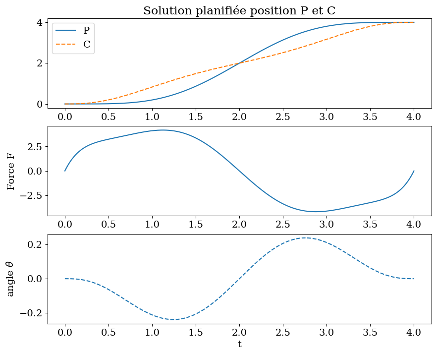
6.3.6. solution planifiée optimale

XXI = XI(tt,XF,TF)
XCX = XC(tt,XF,TF,OMEGA0)
FFX = FX(tt,XF,TF,OMEGA0,ALPHA)
TTHX= THX(tt,XF,TF,OMEGA0,L0)
plt.figure(figsize=(10,8))
plt.subplot(3,1,1)
plt.plot(tt,XXI,label="P")
plt.plot(tt,XCX,'--',label="C")
plt.legend()
plt.title("Solution planifiée position P et C")
plt.subplot(3,1,2)
plt.plot(tt,FFX)
plt.ylabel("Force F")
plt.subplot(3,1,3)
plt.plot(tt,TTHX,'--')
plt.ylabel("angle $\\theta$")
plt.xlabel('t');

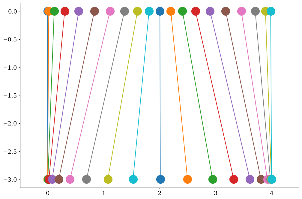
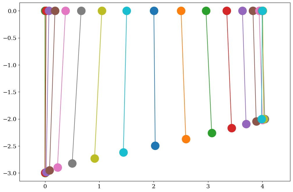
# tracer du mouvement optimal
plt.figure(figsize=(12,8))
for i in range(0,len(tt),20):
    X,Y = [XCX[i],XXI[i]],[0.,-L0]
    plt.plot(X,Y,'-o',ms=20)
plt.axis('equal');

6.3.7. Simulation

display(sp.simplify(LM.rhs()).doit())
smb = sp.simplify(sp.simplify(LM.rhs()).doit().subs({l:l0,g:omega0**2*l0}))
display(smb)
smbF = sp.lambdify([theta,xc,thetap,xcp,Fc,l0,omega0,alpha],smb,'numpy')

\[\begin{split}\displaystyle \left[\begin{matrix}\dot{\theta}\\\dot{x}_{c}\\- \frac{F_{c} \alpha \cos{\left(\theta \right)} + \alpha g \sin{\left(\theta \right)} + g \sin{\left(\theta \right)} + \frac{l_{0} \sin{\left(2 \theta \right)} \dot{\theta}^{2}}{2}}{l_{0} \left(\alpha + \sin^{2}{\left(\theta \right)}\right)}\\\frac{F_{c} \alpha + \frac{g \sin{\left(2 \theta \right)}}{2} + l_{0} \sin{\left(\theta \right)} \dot{\theta}^{2}}{\alpha + \sin^{2}{\left(\theta \right)}}\end{matrix}\right]\end{split}\]

\[\begin{split}\displaystyle \left[\begin{matrix}\dot{\theta}\\\dot{x}_{c}\\\frac{- F_{c} \alpha \cos{\left(\theta \right)} - \alpha l_{0} \omega_{0}^{2} \sin{\left(\theta \right)} - l_{0} \omega_{0}^{2} \sin{\left(\theta \right)} - \frac{l_{0} \sin{\left(2 \theta \right)} \dot{\theta}^{2}}{2}}{l_{0} \left(\alpha + \sin^{2}{\left(\theta \right)}\right)}\\\frac{F_{c} \alpha + \frac{l_{0} \omega_{0}^{2} \sin{\left(2 \theta \right)}}{2} + l_{0} \sin{\left(\theta \right)} \dot{\theta}^{2}}{\alpha + \sin^{2}{\left(\theta \right)}}\end{matrix}\right]\end{split}\]

def Fs(Y,t):
    """commande simple"""
    global L0,OMEGA0,ALPHA,TF,XF
    FC = FCX(t,TF,XF,ALPHA)
    FF = smbF(Y[0],Y[1],Y[2],Y[3],FC,L0,OMEGA0,ALPHA)
    return FF[:,0]
def Fa(Y,t):
    """asservissement simple"""
    global L0,OMEGA0,ALPHA,TF,XF,KC,TC
    FC = FCA(t,TF,XF,Y[1],Y[3],KC,TC)
    FF = smbF(Y[0],Y[1],Y[2],Y[3],FC,L0,OMEGA0,ALPHA)
    return FF[:,0]
def F(Y,t):
    """commande lente couplée"""
    global L0,OMEGA0,ALPHA
    FC = FX(t,XF,TF,OMEGA0,ALPHA)
    FF = smbF(Y[0],Y[1],Y[2],Y[3],FC,L0,OMEGA0,ALPHA)
    return FF[:,0]

from scipy.integrate import odeint
Y0 = [0.0, 0.0, 0., 0. ]
# perturbation
Y0 = [0.01,0.01, 0.,0.]
tt  = np.linspace(0,TF,Nt)
sol = odeint(F,Y0,tt)
sols= odeint(Fs,Y0,tt)
sola= odeint(Fa,Y0,tt)
THETA = sol[:,0]
XXC   = sol[:,1]
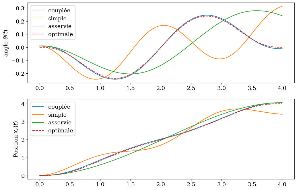
print("Erreur sur la position finale")
print("commande couplée  erreur xc={:.4f} \t theta={:.3f} deg".format(sol[-1,1]-XF ,np.degrees(sol[-1,0])))
print("commande simple   erreur xc={:.4f} \t theta={:.3f} deg".format(sols[-1,1]-XF,np.degrees(sols[-1,0])))
print("commande asservie erreur xc={:.4f} \t theta={:.3f} deg".format(sola[-1,1]-XF,np.degrees(sola[-1,0])))

Erreur sur la position finale
commande couplée  erreur xc=0.0525 	 theta=-0.645 deg
commande simple   erreur xc=-0.5876 	 theta=17.988 deg
commande asservie erreur xc=0.0652 	 theta=13.829 deg

plt.figure(figsize=(12,8))
plt.subplot(2,1,1)
plt.plot(tt,THETA,label="couplée")
plt.plot(tt,sols[:,0],label="simple")
plt.plot(tt,sola[:,0],label="asservie")
plt.plot(tt,TTHX,'--',label="optimale")
plt.ylabel('angle $\\theta(t)$')
plt.legend();
plt.subplot(2,1,2)
plt.plot(tt,XXC,label="couplée")
plt.plot(tt,sols[:,1],label="simple")
plt.plot(tt,sola[:,1],label="asservie")
plt.plot(tt,XCX,'--',label="optimale")
plt.ylabel('Position $x_c(t)$')
plt.legend();

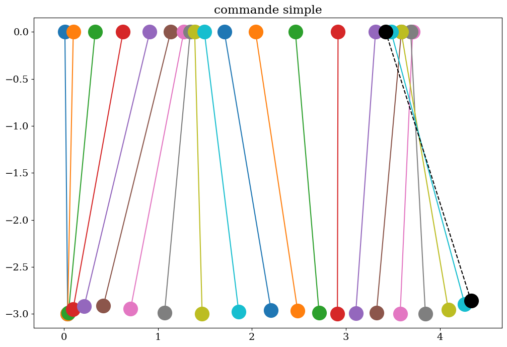
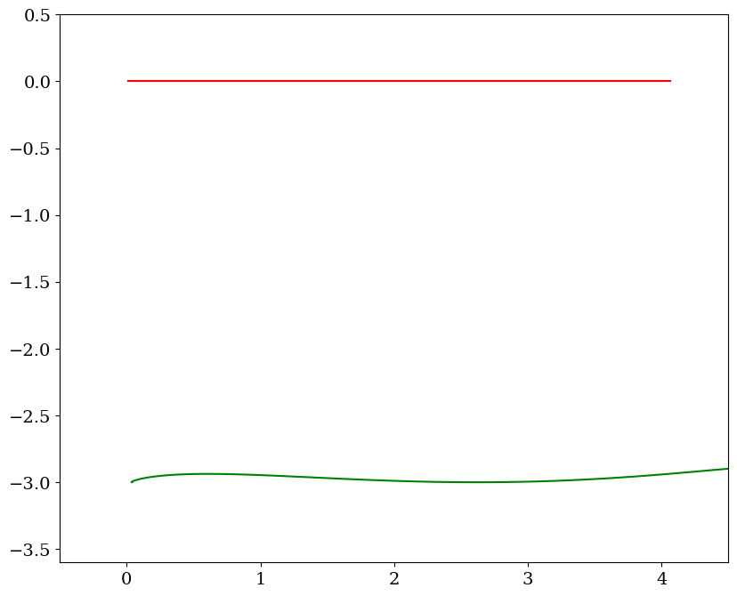
# tracer du mouvement cde simple
pas = 5
chariots = Chariot(L0,sols[::pas,1],sols[::pas,0],tt[pas])
chariots.trace(titre="commande simple",pas=4)

# animation
anims = chariots.calculanim(-0.5, XF+0.5, -1.2*L0, 0.5)

plt.rc('animation', html='jshtml')
anims

Once Loop Reflect

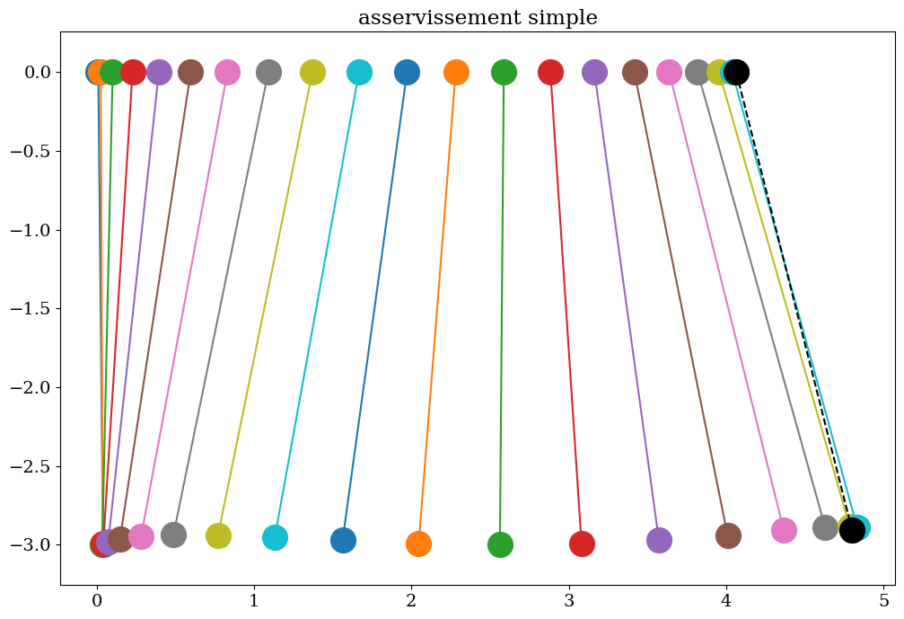
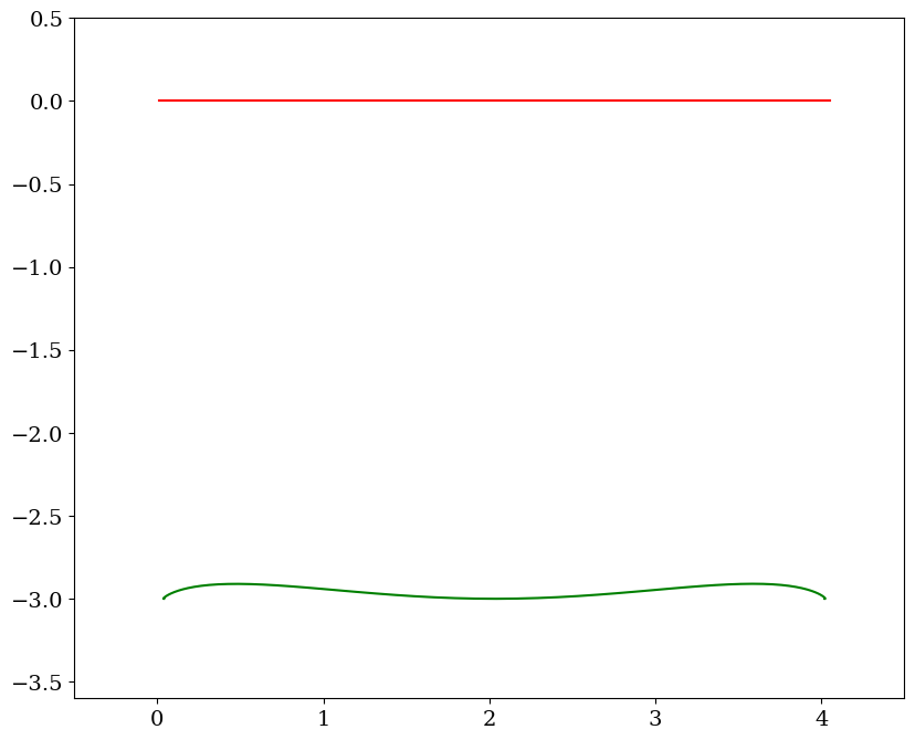
# tracer du mouvement asservisement
chariota = Chariot(L0,sola[::pas,1],sola[::pas,0],tt[pas])
chariota.trace(titre="asservissement simple",pas=4)

# animation
anima = chariota.calculanim(-0.5, XF+0.5, -1.2*L0, 0.5)

plt.rc('animation', html='jshtml')
anima

Once Loop Reflect

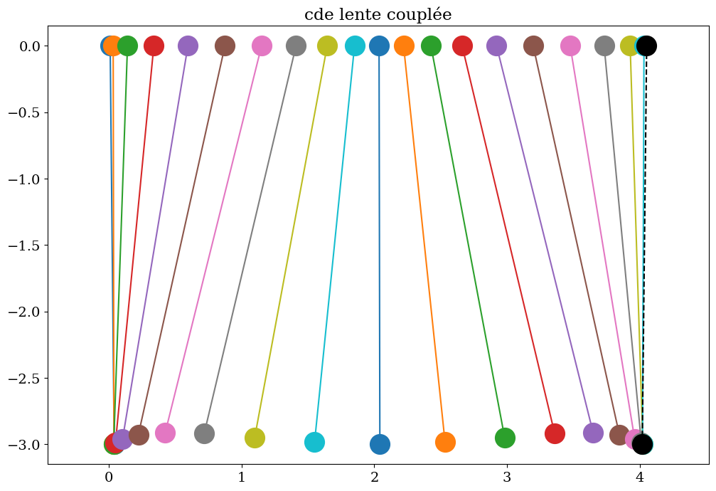
# tracer du mouvement cde lente couplee
chariotc = Chariot(L0,XXC[::pas],THETA[::pas],tt[pas])
chariotc.trace(titre="cde lente couplée",pas=4)

# animation
animc = chariotc.calculanim(-0.5, XF+0.5, -1.2*L0, 0.5)

plt.rc('animation', html='jshtml')
animc

Once Loop Reflect

6.4. Asservissement: regulateur bas niveau

pour rendre la commande précédente robuste on ajoute un asservissement pour suivre la trajectoire idéale

• trajectoire imposée \(x_i(t)\) à partir de \(\xi(t)\) $\(x_i(t) = \xi + \frac{l_0}{g} \ddot{\xi}\)$

• commande asservissement (ajout à la commande idéale précédente) $\( F_c = F_i -K_c ( (x_c-x_i) + T_c(\dot{x_c}-\dot{x_i})) \)$

smb = sp.simplify(LM.rhs().subs({g:omega0**2*l0}))
display(smb)

\[\begin{split}\displaystyle \left[\begin{matrix}\dot{\theta}\\\dot{x}_{c}\\- \frac{F_{c} \alpha \cos{\left(\theta \right)} + \alpha l_{0} \omega_{0}^{2} \sin{\left(\theta \right)} + l_{0} \omega_{0}^{2} \sin{\left(\theta \right)} + \frac{l_{0} \sin{\left(2 \theta \right)} \dot{\theta}^{2}}{2}}{l_{0} \left(\alpha + \sin^{2}{\left(\theta \right)}\right)}\\\frac{F_{c} \alpha + \frac{l_{0} \omega_{0}^{2} \sin{\left(2 \theta \right)}}{2} + l_{0} \sin{\left(\theta \right)} \dot{\theta}^{2}}{\alpha + \sin^{2}{\left(\theta \right)}}\end{matrix}\right]\end{split}\]

display(xcx)
Kc, Tc = sp.symbols('K_c T_c')
Fca = -Kc*((xc-xcx)+(xcp-xcx.diff(t,1))*Tc)
display(Fca)

\[\displaystyle \frac{t^{3} x_{f} \left(70 \omega_{0}^{2} t^{6} - 315 \omega_{0}^{2} t^{5} t_{f} + 540 \omega_{0}^{2} t^{4} t_{f}^{2} - 420 \omega_{0}^{2} t^{3} t_{f}^{3} + 126 \omega_{0}^{2} t^{2} t_{f}^{4} + 5040 t^{4} - 17640 t^{3} t_{f} + 22680 t^{2} t_{f}^{2} - 12600 t t_{f}^{3} + 2520 t_{f}^{4}\right)}{\omega_{0}^{2} t_{f}^{9}}\]

\[\displaystyle - K_{c} \left(T_{c} \left(\dot{x}_{c} - \frac{t^{3} x_{f} \left(420 \omega_{0}^{2} t^{5} - 1575 \omega_{0}^{2} t^{4} t_{f} + 2160 \omega_{0}^{2} t^{3} t_{f}^{2} - 1260 \omega_{0}^{2} t^{2} t_{f}^{3} + 252 \omega_{0}^{2} t t_{f}^{4} + 20160 t^{3} - 52920 t^{2} t_{f} + 45360 t t_{f}^{2} - 12600 t_{f}^{3}\right)}{\omega_{0}^{2} t_{f}^{9}} - \frac{3 t^{2} x_{f} \left(70 \omega_{0}^{2} t^{6} - 315 \omega_{0}^{2} t^{5} t_{f} + 540 \omega_{0}^{2} t^{4} t_{f}^{2} - 420 \omega_{0}^{2} t^{3} t_{f}^{3} + 126 \omega_{0}^{2} t^{2} t_{f}^{4} + 5040 t^{4} - 17640 t^{3} t_{f} + 22680 t^{2} t_{f}^{2} - 12600 t t_{f}^{3} + 2520 t_{f}^{4}\right)}{\omega_{0}^{2} t_{f}^{9}}\right) + x_{c} - \frac{t^{3} x_{f} \left(70 \omega_{0}^{2} t^{6} - 315 \omega_{0}^{2} t^{5} t_{f} + 540 \omega_{0}^{2} t^{4} t_{f}^{2} - 420 \omega_{0}^{2} t^{3} t_{f}^{3} + 126 \omega_{0}^{2} t^{2} t_{f}^{4} + 5040 t^{4} - 17640 t^{3} t_{f} + 22680 t^{2} t_{f}^{2} - 12600 t t_{f}^{3} + 2520 t_{f}^{4}\right)}{\omega_{0}^{2} t_{f}^{9}}\right)\]

smbF = sp.lambdify([theta,xc,thetap,xcp,l0,omega0,alpha,Fc],smb)
FCa  = sp.lambdify([t,xc,xcp,tf,xf,omega0,Kc,Tc],Fca)

6.4.1. Simulation

# parametres
def F(Y,t):
    global TF,XF,L0,OMEGA0,ALPHA,KC,TC
    FC = 0
    # cde idéale
    FC += FX(t,XF,TF,OMEGA0,ALPHA)
    # asservissement
    FC += FCa(t,Y[1],Y[3],TF,XF,OMEGA0,KC,TC)
    # 2nd membre
    FF = smbF(Y[0],Y[1],Y[2],Y[3],L0,OMEGA0,ALPHA,FC)
    return FF[:,0]

# parametres
KC = 200
TC = np.sqrt(4/KC)
print("parametres:",KC,TC,TF)
# simulation
Y0 = [0.0, 0.0, 0., 0. ]
# perturbation
Y0 = [0.01,0.01,0.,0.]
sol = odeint(F,Y0,tt)
THETA = sol[:,0]
XXC   = sol[:,1]
print("Erreur sur la position finale")
print("commande couplée  erreur xc={:.3f} \t theta={:.3f} deg".format(sol[-1,1]-XF ,np.degrees(sol[-1,0])))

parametres: 200 0.1414213562373095 4.0
Erreur sur la position finale
commande couplée  erreur xc=0.002 	 theta=0.849 deg

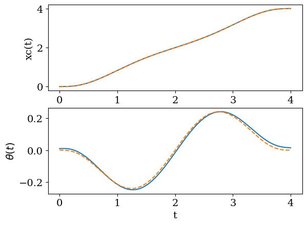
plt.subplot(2,1,1)
plt.plot(tt,XXC)
plt.plot(tt,XCX,'--')
plt.ylabel("xc(t)")
plt.subplot(2,1,2)
plt.plot(tt,THETA)
plt.plot(tt,TTHX,'--')
plt.ylabel("$\\theta(t)$")
plt.xlabel('t');

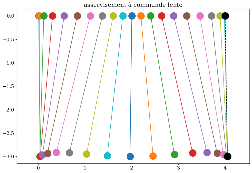
chariot = Chariot(L0,XXC[::pas],THETA[::pas],tt[pas])
chariot.trace(titre="asservisement à commande lente",pas=4)

anim = chariot.calculanim(-0.5, XF+0.5, -1.2*L0, 0.5)

plt.rc('animation', html='jshtml')
anim

Once Loop Reflect

6.5. cas avec une longueur différence

6.5.1. mouvement de la charge

• coordonnees \(\xi(t)\), \(\eta(t)\) dans le repere fixe (voir cours) $\(\xi = l \sin\theta + x-c \)\( \)\(\eta = -l \cos\theta \)$

• équations d’équilibre $\( m\ddot\xi = -T \sin\theta\)\( \)\( m\ddot\xi = -T \sin\theta\)$

• d’où l’expression de \(\theta\), \(l\) et \(x_c\) en fonction de \(\xi\) et \(\eta\)

\[ \tan \theta = \frac{\ddot{\xi}}{\ddot{\eta}-g}\]

\[ x_c = \xi - \frac{\eta\ddot{\xi}}{\ddot{\eta}-g}\]

\[ (\xi - x_c)^2 + \eta^2 = l^2 \]

• trajectoire idéale

on planifie une trajectoire idéale pour \(\xi\) et \(\eta\) , et on en déduit la valeur de \(x_c(t)\) \(\theta(t)\) et \(l(t)\), et le contrôle assoicié

xi, eta = dynamicsymbols('xi eta')
display(sp.Eq(sp.tan(theta), xi.diff(t,t)/(eta.diff(t,t)-g)))
display(sp.Eq(xc, xi - eta*xi.diff(t,t)/(eta.diff(t,t)-g)) )

\[\displaystyle \tan{\left(\theta \right)} = \frac{\ddot{\xi}}{- g + \ddot{\eta}}\]

\[\displaystyle x_{c} = \xi - \frac{\eta \ddot{\xi}}{- g + \ddot{\eta}}\]

6.5.1.1. trajectoire planifiée

trajectoire \(\xi(t)\) tq. $\(\xi(0)=0, \frac{d\xi}{dt}(0)=0, \frac{d^2\xi}{dt^2}(0)=0, \frac{d^3\xi}{dt^3}(0)=0, \frac{d^4\xi}{dt^4}(0)=0\)\( \)\(\xi(t_f)=x_f, \frac{d\xi}{dt}(t_f)=0, \frac{d^2\xi}{dt^2}(t_f)=0, \frac{d^3\xi}{dt^3}(t_f)=0, \frac{d^4\xi}{dt^4}(t_f)=0\)$

• \(\xi(t)\) polynome de degré 9 en t

trajectoire \(\eta(t)\) (même condition que \(\xi\)) sauf sur la position

• \(\eta=-l_0\) longueur à \(t=0\)

• \(\eta=-l_f\) longueur à \(t=t_f\)

xf, tf = sp.symbols('x_f t_f')
x = xf*(t/tf)**5*(126-420*(t/tf)+540*(t/tf)**2-315*(t/tf)**3+70*(t/tf)**4)
display(sp.Eq(xi,x))
# verification
print("dérivées en tf:",x.diff(t,1).subs({t:tf}),x.diff(t,2).subs({t:tf}),x.diff(t,3).subs({t:tf}),x.diff(t,4).subs({t:tf}))

\[\displaystyle \xi = \frac{t^{5} x_{f} \left(\frac{70 t^{4}}{t_{f}^{4}} - \frac{315 t^{3}}{t_{f}^{3}} + \frac{540 t^{2}}{t_{f}^{2}} - \frac{420 t}{t_{f}} + 126\right)}{t_{f}^{5}}\]

dérivées en tf: 0 0 0 0

lf = sp.symbols('l_f')
y = - l0 - (lf - l0)*(x/xf)
display(sp.Eq(eta,y))

\[\displaystyle \eta = - l_{0} - \frac{t^{5} \left(- l_{0} + l_{f}\right) \left(\frac{70 t^{4}}{t_{f}^{4}} - \frac{315 t^{3}}{t_{f}^{3}} + \frac{540 t^{2}}{t_{f}^{2}} - \frac{420 t}{t_{f}} + 126\right)}{t_{f}^{5}}\]

6.5.2. cas linéaire

on suppose que \(\theta \approx 0\)

trajectoire idéale du chariot et du cable : $\(x_{ref}(t) \approx \xi(t) \)\( \)\(l_{ref}(t) \approx - \eta(t)\)$

d’ou l’asservissement de \(F_c\) et \(C_t\)

\[ F_c = -K_c ( (x-x_{ref}) + T_c (\dot{x}-\dot{x}_{ref})) \]

\[ C_t = -g -K_t ( (l-l_{ref}) + T_t (\dot{l}-\dot{l}_{ref})) \]

xref = x
lref = -y
display(xref, lref)

\[\displaystyle \frac{t^{5} x_{f} \left(\frac{70 t^{4}}{t_{f}^{4}} - \frac{315 t^{3}}{t_{f}^{3}} + \frac{540 t^{2}}{t_{f}^{2}} - \frac{420 t}{t_{f}} + 126\right)}{t_{f}^{5}}\]

\[\displaystyle l_{0} + \frac{t^{5} \left(- l_{0} + l_{f}\right) \left(\frac{70 t^{4}}{t_{f}^{4}} - \frac{315 t^{3}}{t_{f}^{3}} + \frac{540 t^{2}}{t_{f}^{2}} - \frac{420 t}{t_{f}} + 126\right)}{t_{f}^{5}}\]

# asservissement
Kc, Tc = sp.symbols('K_c T_c')
Fca = -Kc*((xc-xref)+(xcp-xref.diff(t,1))*Tc)
Fca = Fca.simplify()
display(Fca)
Kt, Tt = sp.symbols('K_t T_t')
Cta = -g -Kt*((l-lref)+(lp-lref.diff(t,1))*Tt)
Cta = Cta.simplify()
display(Cta)

\[\displaystyle \frac{K_{c} \left(630 T_{c} t^{8} x_{f} - 2520 T_{c} t^{7} t_{f} x_{f} + 3780 T_{c} t^{6} t_{f}^{2} x_{f} - 2520 T_{c} t^{5} t_{f}^{3} x_{f} + 630 T_{c} t^{4} t_{f}^{4} x_{f} - T_{c} t_{f}^{9} \dot{x}_{c} + 70 t^{9} x_{f} - 315 t^{8} t_{f} x_{f} + 540 t^{7} t_{f}^{2} x_{f} - 420 t^{6} t_{f}^{3} x_{f} + 126 t^{5} t_{f}^{4} x_{f} - t_{f}^{9} x_{c}\right)}{t_{f}^{9}}\]

\[\displaystyle \frac{K_{t} \left(- T_{t} \left(5 t^{5} \left(l_{0} - l_{f}\right) \left(56 t^{3} - 189 t^{2} t_{f} + 216 t t_{f}^{2} - 84 t_{f}^{3}\right) + 5 t^{4} \left(l_{0} - l_{f}\right) \left(70 t^{4} - 315 t^{3} t_{f} + 540 t^{2} t_{f}^{2} - 420 t t_{f}^{3} + 126 t_{f}^{4}\right) + t_{f}^{9} \dot{l}\right) - t^{5} \left(l_{0} - l_{f}\right) \left(70 t^{4} - 315 t^{3} t_{f} + 540 t^{2} t_{f}^{2} - 420 t t_{f}^{3} + 126 t_{f}^{4}\right) + t_{f}^{9} \left(l_{0} - l\right)\right) - g t_{f}^{9}}{t_{f}^{9}}\]

# fct python
FCa = sp.lambdify([t,xc,xcp,xf,tf,Kc,Tc],Fca,'numpy')
CTa = sp.lambdify([t,l,lp,l0,lf,tf,Kt,Tt,g],Cta,'numpy')
Xref= sp.lambdify([t,xf,tf],xref,'numpy')
Lref= sp.lambdify([t,l0,lf,tf],lref,'numpy')

6.5.3. Equation lagrange avec couple

alpha = sp.Symbol('alpha')
La = sp.simplify(La.subs({M:alpha*m}))
display(La)
Fc, Ct = sp.symbols('F_c C_t')
LM = LagrangesMethod(La,[theta,xc,l],forcelist=[(C,Fc*alpha*m*RO.x),(Rt,Ct*m*rho*RO.z)], frame = RO)
eq = sp.simplify(LM.form_lagranges_equations())
display(eq)

\[\displaystyle \frac{m \left(\alpha \dot{x}_{c}^{2} + 2 g l \cos{\left(\theta \right)} + l^{2} \dot{\theta}^{2} + 2 l \cos{\left(\theta \right)} \dot{\theta} \dot{x}_{c} + 2 \sin{\left(\theta \right)} \dot{l} \dot{x}_{c} + \dot{l}^{2} + \dot{x}_{c}^{2}\right)}{2}\]

\[\begin{split}\displaystyle \left[\begin{matrix}m \left(g \sin{\left(\theta \right)} + l \ddot{\theta} + \cos{\left(\theta \right)} \ddot{x}_{c} + 2 \dot{l} \dot{\theta}\right) l\\m \left(- F_{c} \alpha + \alpha \ddot{x}_{c} - l \sin{\left(\theta \right)} \dot{\theta}^{2} + l \cos{\left(\theta \right)} \ddot{\theta} + \sin{\left(\theta \right)} \ddot{l} + 2 \cos{\left(\theta \right)} \dot{l} \dot{\theta} + \ddot{x}_{c}\right)\\m \left(- C_{t} - g \cos{\left(\theta \right)} - l \dot{\theta}^{2} + \sin{\left(\theta \right)} \ddot{x}_{c} + \ddot{l}\right)\end{matrix}\right]\end{split}\]

smb = sp.simplify(sp.simplify(LM.rhs()).doit())
display(smb)
smbF = sp.lambdify([theta,xc,l,thetap,xcp,lp,Fc,Ct,g,alpha],smb,'numpy')

\[\begin{split}\displaystyle \left[\begin{matrix}\dot{\theta}\\\dot{x}_{c}\\\dot{l}\\\frac{\frac{C_{t} \sin{\left(2 \theta \right)}}{2} - F_{c} \alpha \cos{\left(\theta \right)} - \alpha g \sin{\left(\theta \right)} - 2 \alpha \dot{l} \dot{\theta}}{\alpha l}\\- \frac{C_{t} \sin{\left(\theta \right)}}{\alpha} + F_{c}\\C_{t} + \frac{C_{t} \sin^{2}{\left(\theta \right)}}{\alpha} - F_{c} \sin{\left(\theta \right)} + g \cos{\left(\theta \right)} + l \dot{\theta}^{2}\end{matrix}\right]\end{split}\]

6.5.4. simulation

# PARAMETRES NUMERIQUES
TF = 10.0
#TF = 8.0
XF = 4.0
ALPHA = 0.5
L0 = 3.0
LF = 2.0
GG = 9.81
KC = 50.0
TC = 20./KC
KT = 50.0
TT = 20./KT
Nt = 400
tt = np.linspace(0,TF,Nt)

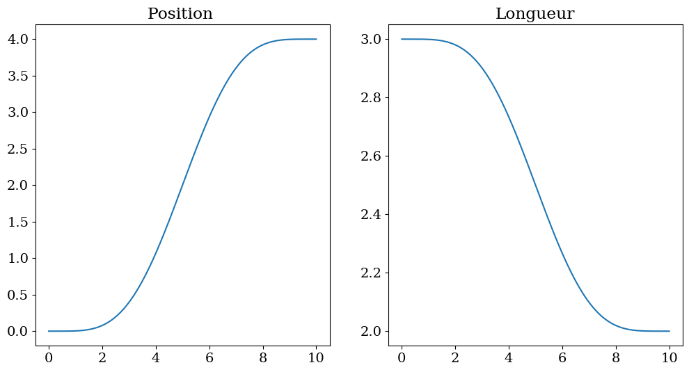
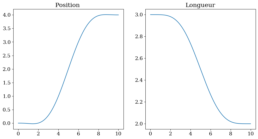
# trajectoire idéale
XREF = Xref(tt,XF,TF)
LREF = Lref(tt,L0,LF,TF)
plt.figure(figsize=(12,6))
plt.subplot(1,2,1)
plt.plot(tt,XREF)
plt.title("Position ")
plt.subplot(1,2,2)
plt.plot(tt,LREF)
plt.title("Longueur")

Text(0.5, 1.0, 'Longueur')

# simulation mouvement
def F(Y,t):
    global ALPHA,TF,XF
    FC = FCa(t,Y[1],Y[4],XF,TF,KC,TC)
    CT = CTa(t,Y[2],Y[5],L0,LF,TF,KT,TT,GG)
    FF = smbF(Y[0],Y[1],Y[2],Y[3],Y[4],Y[5],FC,CT,GG,ALPHA)
    return FF[:,0]

Y0 = [0.0, 0.0, L0, 0., 0., 0. ]
sol = odeint(F,Y0,tt)
THETA = sol[:,0]
XC    = sol[:,1]
LL    = sol[:,2]

plt.figure(figsize=(12,6))
plt.subplot(1,3,1)
plt.plot(tt,THETA*180/np.pi)
plt.ylim(-10,10)
plt.title("Angle$\\theta$ en degré")
plt.subplot(1,3,2)
plt.plot(tt,XC)
plt.plot(tt,XREF,'--')
plt.title('Position $x_c(t)$')
plt.subplot(1,3,3)
plt.plot(tt,LL)
plt.plot(tt,LREF,'--')
plt.title('longueur $l(t)$')

Text(0.5, 1.0, 'longueur $l(t)$')

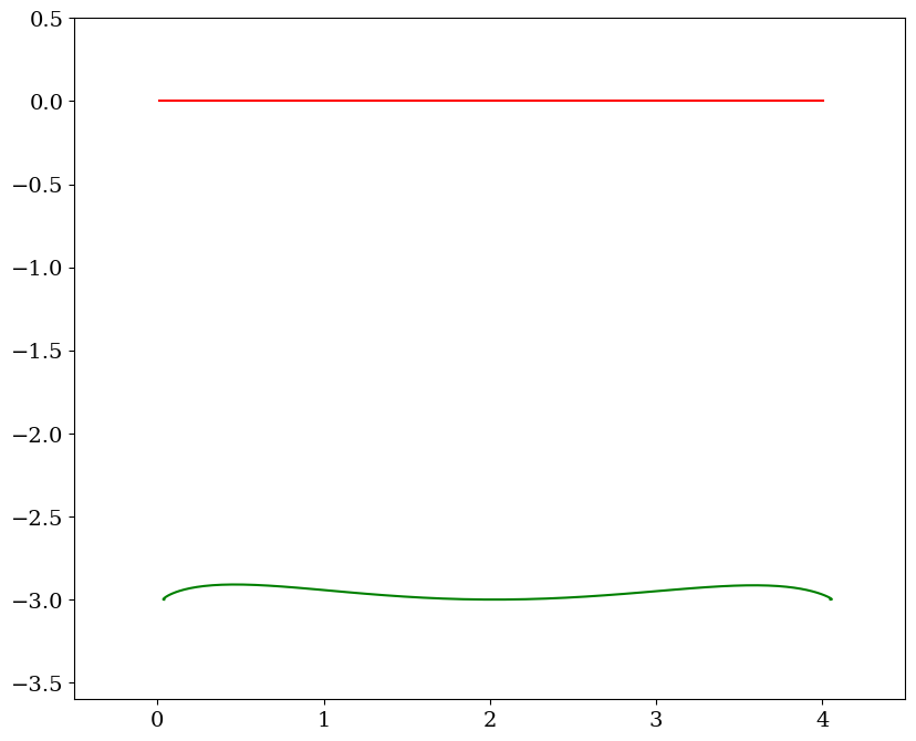
# tracer du mouvement
plt.figure(figsize=(12,8))
for i in range(0,len(tt),20):
    X,Y = [XC[i],XC[i]+LL[i]*np.sin(THETA[i])],[0.,-LL[i]*np.cos(THETA[i])]
    plt.plot(X,Y,'-o',ms=20)
plt.axis('equal')

\[\displaystyle \left( -0.202291418357987, \ 4.24811978551773, \ -3.15, \ 0.15\right)\]

6.5.5. cas non linéaire

• ddl fonction de la trajectoire (idéale) \(\xi\) \(\eta\) $\( x_{ref} = \xi - \frac{\eta\ddot{\xi}}{\ddot{\eta}-g}\)$

\[ l_{ref} = \sqrt{(\frac{\eta\ddot{\xi}}{\ddot{\eta}-g})^2 + \eta^2}\]

xref = x - y*x.diff(t,2)/(y.diff(t,2)-g)
xref = xref.doit()
lref = sp.sqrt((y*x.diff(t,2)/(y.diff(t,2)-g))**2 + y**2)
lref = lref.doit()
print(xref, lref)

t**5*x_f*(70*t**4/t_f**4 - 315*t**3/t_f**3 + 540*t**2/t_f**2 - 420*t/t_f + 126)/t_f**5 - 10*t**3*x_f*(-l_0 - t**5*(-l_0 + l_f)*(70*t**4/t_f**4 - 315*t**3/t_f**3 + 540*t**2/t_f**2 - 420*t/t_f + 126)/t_f**5)*(140*t**4/t_f**4 - 630*t**3/t_f**3 + 3*t**2*(28*t**2/t_f**2 - 63*t/t_f + 36)/t_f**2 + 1080*t**2/t_f**2 + 5*t*(56*t**3/t_f**3 - 189*t**2/t_f**2 + 216*t/t_f - 84)/t_f - 840*t/t_f + 252)/(t_f**5*(-g + 10*t**3*(l_0 - l_f)*(140*t**4/t_f**4 - 630*t**3/t_f**3 + 3*t**2*(28*t**2/t_f**2 - 63*t/t_f + 36)/t_f**2 + 1080*t**2/t_f**2 + 5*t*(56*t**3/t_f**3 - 189*t**2/t_f**2 + 216*t/t_f - 84)/t_f - 840*t/t_f + 252)/t_f**5)) sqrt(100*t**6*x_f**2*(-l_0 - t**5*(-l_0 + l_f)*(70*t**4/t_f**4 - 315*t**3/t_f**3 + 540*t**2/t_f**2 - 420*t/t_f + 126)/t_f**5)**2*(140*t**4/t_f**4 - 630*t**3/t_f**3 + 3*t**2*(28*t**2/t_f**2 - 63*t/t_f + 36)/t_f**2 + 1080*t**2/t_f**2 + 5*t*(56*t**3/t_f**3 - 189*t**2/t_f**2 + 216*t/t_f - 84)/t_f - 840*t/t_f + 252)**2/(t_f**10*(-g + 10*t**3*(l_0 - l_f)*(140*t**4/t_f**4 - 630*t**3/t_f**3 + 3*t**2*(28*t**2/t_f**2 - 63*t/t_f + 36)/t_f**2 + 1080*t**2/t_f**2 + 5*t*(56*t**3/t_f**3 - 189*t**2/t_f**2 + 216*t/t_f - 84)/t_f - 840*t/t_f + 252)/t_f**5)**2) + (-l_0 - t**5*(-l_0 + l_f)*(70*t**4/t_f**4 - 315*t**3/t_f**3 + 540*t**2/t_f**2 - 420*t/t_f + 126)/t_f**5)**2)

# asservissement pour obtenir la trajectoire
Kc, Tc = sp.symbols('K_c T_c')
Fca = -Kc*((xc-xref)+(xcp-xref.diff(t,1))*Tc)
#Fca = Fca.simplify()
#display(Fca)
print(Fca)
Kt, Tt = sp.symbols('K_t T_t')
Cta = -g - Kt*((l-lref)+(lp-lref.diff(t,1))*Tt)
#Cta = Cta.simplify()
#display(Cta)
print(Cta)

-K_c*(T_c*(-t**5*x_f*(280*t**3/t_f**4 - 945*t**2/t_f**3 + 1080*t/t_f**2 - 420/t_f)/t_f**5 - 5*t**4*x_f*(70*t**4/t_f**4 - 315*t**3/t_f**3 + 540*t**2/t_f**2 - 420*t/t_f + 126)/t_f**5 + 10*t**3*x_f*(-l_0 - t**5*(-l_0 + l_f)*(70*t**4/t_f**4 - 315*t**3/t_f**3 + 540*t**2/t_f**2 - 420*t/t_f + 126)/t_f**5)*(560*t**3/t_f**4 + 3*t**2*(56*t/t_f**2 - 63/t_f)/t_f**2 - 1890*t**2/t_f**3 + 5*t*(168*t**2/t_f**3 - 378*t/t_f**2 + 216/t_f)/t_f + 6*t*(28*t**2/t_f**2 - 63*t/t_f + 36)/t_f**2 + 2160*t/t_f**2 + 5*(56*t**3/t_f**3 - 189*t**2/t_f**2 + 216*t/t_f - 84)/t_f - 840/t_f)/(t_f**5*(-g + 10*t**3*(l_0 - l_f)*(140*t**4/t_f**4 - 630*t**3/t_f**3 + 3*t**2*(28*t**2/t_f**2 - 63*t/t_f + 36)/t_f**2 + 1080*t**2/t_f**2 + 5*t*(56*t**3/t_f**3 - 189*t**2/t_f**2 + 216*t/t_f - 84)/t_f - 840*t/t_f + 252)/t_f**5)) + 10*t**3*x_f*(-t**5*(-l_0 + l_f)*(280*t**3/t_f**4 - 945*t**2/t_f**3 + 1080*t/t_f**2 - 420/t_f)/t_f**5 - 5*t**4*(-l_0 + l_f)*(70*t**4/t_f**4 - 315*t**3/t_f**3 + 540*t**2/t_f**2 - 420*t/t_f + 126)/t_f**5)*(140*t**4/t_f**4 - 630*t**3/t_f**3 + 3*t**2*(28*t**2/t_f**2 - 63*t/t_f + 36)/t_f**2 + 1080*t**2/t_f**2 + 5*t*(56*t**3/t_f**3 - 189*t**2/t_f**2 + 216*t/t_f - 84)/t_f - 840*t/t_f + 252)/(t_f**5*(-g + 10*t**3*(l_0 - l_f)*(140*t**4/t_f**4 - 630*t**3/t_f**3 + 3*t**2*(28*t**2/t_f**2 - 63*t/t_f + 36)/t_f**2 + 1080*t**2/t_f**2 + 5*t*(56*t**3/t_f**3 - 189*t**2/t_f**2 + 216*t/t_f - 84)/t_f - 840*t/t_f + 252)/t_f**5)) + 10*t**3*x_f*(-l_0 - t**5*(-l_0 + l_f)*(70*t**4/t_f**4 - 315*t**3/t_f**3 + 540*t**2/t_f**2 - 420*t/t_f + 126)/t_f**5)*(-10*t**3*(l_0 - l_f)*(560*t**3/t_f**4 + 3*t**2*(56*t/t_f**2 - 63/t_f)/t_f**2 - 1890*t**2/t_f**3 + 5*t*(168*t**2/t_f**3 - 378*t/t_f**2 + 216/t_f)/t_f + 6*t*(28*t**2/t_f**2 - 63*t/t_f + 36)/t_f**2 + 2160*t/t_f**2 + 5*(56*t**3/t_f**3 - 189*t**2/t_f**2 + 216*t/t_f - 84)/t_f - 840/t_f)/t_f**5 - 30*t**2*(l_0 - l_f)*(140*t**4/t_f**4 - 630*t**3/t_f**3 + 3*t**2*(28*t**2/t_f**2 - 63*t/t_f + 36)/t_f**2 + 1080*t**2/t_f**2 + 5*t*(56*t**3/t_f**3 - 189*t**2/t_f**2 + 216*t/t_f - 84)/t_f - 840*t/t_f + 252)/t_f**5)*(140*t**4/t_f**4 - 630*t**3/t_f**3 + 3*t**2*(28*t**2/t_f**2 - 63*t/t_f + 36)/t_f**2 + 1080*t**2/t_f**2 + 5*t*(56*t**3/t_f**3 - 189*t**2/t_f**2 + 216*t/t_f - 84)/t_f - 840*t/t_f + 252)/(t_f**5*(-g + 10*t**3*(l_0 - l_f)*(140*t**4/t_f**4 - 630*t**3/t_f**3 + 3*t**2*(28*t**2/t_f**2 - 63*t/t_f + 36)/t_f**2 + 1080*t**2/t_f**2 + 5*t*(56*t**3/t_f**3 - 189*t**2/t_f**2 + 216*t/t_f - 84)/t_f - 840*t/t_f + 252)/t_f**5)**2) + 30*t**2*x_f*(-l_0 - t**5*(-l_0 + l_f)*(70*t**4/t_f**4 - 315*t**3/t_f**3 + 540*t**2/t_f**2 - 420*t/t_f + 126)/t_f**5)*(140*t**4/t_f**4 - 630*t**3/t_f**3 + 3*t**2*(28*t**2/t_f**2 - 63*t/t_f + 36)/t_f**2 + 1080*t**2/t_f**2 + 5*t*(56*t**3/t_f**3 - 189*t**2/t_f**2 + 216*t/t_f - 84)/t_f - 840*t/t_f + 252)/(t_f**5*(-g + 10*t**3*(l_0 - l_f)*(140*t**4/t_f**4 - 630*t**3/t_f**3 + 3*t**2*(28*t**2/t_f**2 - 63*t/t_f + 36)/t_f**2 + 1080*t**2/t_f**2 + 5*t*(56*t**3/t_f**3 - 189*t**2/t_f**2 + 216*t/t_f - 84)/t_f - 840*t/t_f + 252)/t_f**5)) + Derivative(x_c(t), t)) - t**5*x_f*(70*t**4/t_f**4 - 315*t**3/t_f**3 + 540*t**2/t_f**2 - 420*t/t_f + 126)/t_f**5 + 10*t**3*x_f*(-l_0 - t**5*(-l_0 + l_f)*(70*t**4/t_f**4 - 315*t**3/t_f**3 + 540*t**2/t_f**2 - 420*t/t_f + 126)/t_f**5)*(140*t**4/t_f**4 - 630*t**3/t_f**3 + 3*t**2*(28*t**2/t_f**2 - 63*t/t_f + 36)/t_f**2 + 1080*t**2/t_f**2 + 5*t*(56*t**3/t_f**3 - 189*t**2/t_f**2 + 216*t/t_f - 84)/t_f - 840*t/t_f + 252)/(t_f**5*(-g + 10*t**3*(l_0 - l_f)*(140*t**4/t_f**4 - 630*t**3/t_f**3 + 3*t**2*(28*t**2/t_f**2 - 63*t/t_f + 36)/t_f**2 + 1080*t**2/t_f**2 + 5*t*(56*t**3/t_f**3 - 189*t**2/t_f**2 + 216*t/t_f - 84)/t_f - 840*t/t_f + 252)/t_f**5)) + x_c(t))
-K_t*(T_t*(Derivative(l(t), t) - (50*t**6*x_f**2*(-l_0 - t**5*(-l_0 + l_f)*(70*t**4/t_f**4 - 315*t**3/t_f**3 + 540*t**2/t_f**2 - 420*t/t_f + 126)/t_f**5)**2*(140*t**4/t_f**4 - 630*t**3/t_f**3 + 3*t**2*(28*t**2/t_f**2 - 63*t/t_f + 36)/t_f**2 + 1080*t**2/t_f**2 + 5*t*(56*t**3/t_f**3 - 189*t**2/t_f**2 + 216*t/t_f - 84)/t_f - 840*t/t_f + 252)*(1120*t**3/t_f**4 + 6*t**2*(56*t/t_f**2 - 63/t_f)/t_f**2 - 3780*t**2/t_f**3 + 10*t*(168*t**2/t_f**3 - 378*t/t_f**2 + 216/t_f)/t_f + 12*t*(28*t**2/t_f**2 - 63*t/t_f + 36)/t_f**2 + 4320*t/t_f**2 + 10*(56*t**3/t_f**3 - 189*t**2/t_f**2 + 216*t/t_f - 84)/t_f - 1680/t_f)/(t_f**10*(-g + 10*t**3*(l_0 - l_f)*(140*t**4/t_f**4 - 630*t**3/t_f**3 + 3*t**2*(28*t**2/t_f**2 - 63*t/t_f + 36)/t_f**2 + 1080*t**2/t_f**2 + 5*t*(56*t**3/t_f**3 - 189*t**2/t_f**2 + 216*t/t_f - 84)/t_f - 840*t/t_f + 252)/t_f**5)**2) + 50*t**6*x_f**2*(-l_0 - t**5*(-l_0 + l_f)*(70*t**4/t_f**4 - 315*t**3/t_f**3 + 540*t**2/t_f**2 - 420*t/t_f + 126)/t_f**5)*(-2*t**5*(-l_0 + l_f)*(280*t**3/t_f**4 - 945*t**2/t_f**3 + 1080*t/t_f**2 - 420/t_f)/t_f**5 - 10*t**4*(-l_0 + l_f)*(70*t**4/t_f**4 - 315*t**3/t_f**3 + 540*t**2/t_f**2 - 420*t/t_f + 126)/t_f**5)*(140*t**4/t_f**4 - 630*t**3/t_f**3 + 3*t**2*(28*t**2/t_f**2 - 63*t/t_f + 36)/t_f**2 + 1080*t**2/t_f**2 + 5*t*(56*t**3/t_f**3 - 189*t**2/t_f**2 + 216*t/t_f - 84)/t_f - 840*t/t_f + 252)**2/(t_f**10*(-g + 10*t**3*(l_0 - l_f)*(140*t**4/t_f**4 - 630*t**3/t_f**3 + 3*t**2*(28*t**2/t_f**2 - 63*t/t_f + 36)/t_f**2 + 1080*t**2/t_f**2 + 5*t*(56*t**3/t_f**3 - 189*t**2/t_f**2 + 216*t/t_f - 84)/t_f - 840*t/t_f + 252)/t_f**5)**2) + 50*t**6*x_f**2*(-l_0 - t**5*(-l_0 + l_f)*(70*t**4/t_f**4 - 315*t**3/t_f**3 + 540*t**2/t_f**2 - 420*t/t_f + 126)/t_f**5)**2*(-20*t**3*(l_0 - l_f)*(560*t**3/t_f**4 + 3*t**2*(56*t/t_f**2 - 63/t_f)/t_f**2 - 1890*t**2/t_f**3 + 5*t*(168*t**2/t_f**3 - 378*t/t_f**2 + 216/t_f)/t_f + 6*t*(28*t**2/t_f**2 - 63*t/t_f + 36)/t_f**2 + 2160*t/t_f**2 + 5*(56*t**3/t_f**3 - 189*t**2/t_f**2 + 216*t/t_f - 84)/t_f - 840/t_f)/t_f**5 - 60*t**2*(l_0 - l_f)*(140*t**4/t_f**4 - 630*t**3/t_f**3 + 3*t**2*(28*t**2/t_f**2 - 63*t/t_f + 36)/t_f**2 + 1080*t**2/t_f**2 + 5*t*(56*t**3/t_f**3 - 189*t**2/t_f**2 + 216*t/t_f - 84)/t_f - 840*t/t_f + 252)/t_f**5)*(140*t**4/t_f**4 - 630*t**3/t_f**3 + 3*t**2*(28*t**2/t_f**2 - 63*t/t_f + 36)/t_f**2 + 1080*t**2/t_f**2 + 5*t*(56*t**3/t_f**3 - 189*t**2/t_f**2 + 216*t/t_f - 84)/t_f - 840*t/t_f + 252)**2/(t_f**10*(-g + 10*t**3*(l_0 - l_f)*(140*t**4/t_f**4 - 630*t**3/t_f**3 + 3*t**2*(28*t**2/t_f**2 - 63*t/t_f + 36)/t_f**2 + 1080*t**2/t_f**2 + 5*t*(56*t**3/t_f**3 - 189*t**2/t_f**2 + 216*t/t_f - 84)/t_f - 840*t/t_f + 252)/t_f**5)**3) + 300*t**5*x_f**2*(-l_0 - t**5*(-l_0 + l_f)*(70*t**4/t_f**4 - 315*t**3/t_f**3 + 540*t**2/t_f**2 - 420*t/t_f + 126)/t_f**5)**2*(140*t**4/t_f**4 - 630*t**3/t_f**3 + 3*t**2*(28*t**2/t_f**2 - 63*t/t_f + 36)/t_f**2 + 1080*t**2/t_f**2 + 5*t*(56*t**3/t_f**3 - 189*t**2/t_f**2 + 216*t/t_f - 84)/t_f - 840*t/t_f + 252)**2/(t_f**10*(-g + 10*t**3*(l_0 - l_f)*(140*t**4/t_f**4 - 630*t**3/t_f**3 + 3*t**2*(28*t**2/t_f**2 - 63*t/t_f + 36)/t_f**2 + 1080*t**2/t_f**2 + 5*t*(56*t**3/t_f**3 - 189*t**2/t_f**2 + 216*t/t_f - 84)/t_f - 840*t/t_f + 252)/t_f**5)**2) + (-l_0 - t**5*(-l_0 + l_f)*(70*t**4/t_f**4 - 315*t**3/t_f**3 + 540*t**2/t_f**2 - 420*t/t_f + 126)/t_f**5)*(-2*t**5*(-l_0 + l_f)*(280*t**3/t_f**4 - 945*t**2/t_f**3 + 1080*t/t_f**2 - 420/t_f)/t_f**5 - 10*t**4*(-l_0 + l_f)*(70*t**4/t_f**4 - 315*t**3/t_f**3 + 540*t**2/t_f**2 - 420*t/t_f + 126)/t_f**5)/2)/sqrt(100*t**6*x_f**2*(-l_0 - t**5*(-l_0 + l_f)*(70*t**4/t_f**4 - 315*t**3/t_f**3 + 540*t**2/t_f**2 - 420*t/t_f + 126)/t_f**5)**2*(140*t**4/t_f**4 - 630*t**3/t_f**3 + 3*t**2*(28*t**2/t_f**2 - 63*t/t_f + 36)/t_f**2 + 1080*t**2/t_f**2 + 5*t*(56*t**3/t_f**3 - 189*t**2/t_f**2 + 216*t/t_f - 84)/t_f - 840*t/t_f + 252)**2/(t_f**10*(-g + 10*t**3*(l_0 - l_f)*(140*t**4/t_f**4 - 630*t**3/t_f**3 + 3*t**2*(28*t**2/t_f**2 - 63*t/t_f + 36)/t_f**2 + 1080*t**2/t_f**2 + 5*t*(56*t**3/t_f**3 - 189*t**2/t_f**2 + 216*t/t_f - 84)/t_f - 840*t/t_f + 252)/t_f**5)**2) + (-l_0 - t**5*(-l_0 + l_f)*(70*t**4/t_f**4 - 315*t**3/t_f**3 + 540*t**2/t_f**2 - 420*t/t_f + 126)/t_f**5)**2)) - sqrt(100*t**6*x_f**2*(-l_0 - t**5*(-l_0 + l_f)*(70*t**4/t_f**4 - 315*t**3/t_f**3 + 540*t**2/t_f**2 - 420*t/t_f + 126)/t_f**5)**2*(140*t**4/t_f**4 - 630*t**3/t_f**3 + 3*t**2*(28*t**2/t_f**2 - 63*t/t_f + 36)/t_f**2 + 1080*t**2/t_f**2 + 5*t*(56*t**3/t_f**3 - 189*t**2/t_f**2 + 216*t/t_f - 84)/t_f - 840*t/t_f + 252)**2/(t_f**10*(-g + 10*t**3*(l_0 - l_f)*(140*t**4/t_f**4 - 630*t**3/t_f**3 + 3*t**2*(28*t**2/t_f**2 - 63*t/t_f + 36)/t_f**2 + 1080*t**2/t_f**2 + 5*t*(56*t**3/t_f**3 - 189*t**2/t_f**2 + 216*t/t_f - 84)/t_f - 840*t/t_f + 252)/t_f**5)**2) + (-l_0 - t**5*(-l_0 + l_f)*(70*t**4/t_f**4 - 315*t**3/t_f**3 + 540*t**2/t_f**2 - 420*t/t_f + 126)/t_f**5)**2) + l(t)) - g

# fct numpy
FCa = sp.lambdify([t,xc,xcp,xf,l0,lf,tf,Kc,Tc,g],Fca,'numpy')
CTa = sp.lambdify([t,l,lp,xf,l0,lf,tf,Kt,Tt,g],Cta,'numpy')
Xref= sp.lambdify([t,xf,l0,lf,tf,g],xref,'numpy')
Lref= sp.lambdify([t,xf,l0,lf,tf,g],lref,'numpy')

# trajectoire ideale
XREF = Xref(tt,XF,L0,LF,TF,GG)
LREF = Lref(tt,XF,L0,LF,TF,GG)
plt.figure(figsize=(12,6))
plt.subplot(1,2,1)
plt.plot(tt,XREF)
plt.title("Position ")
plt.subplot(1,2,2)
plt.plot(tt,LREF)
plt.title("Longueur")

Text(0.5, 1.0, 'Longueur')

# simulation mouvement
def F(Y,t):
    global ALPHA,TF,XF
    FC = FCa(t,Y[1],Y[4],XF,L0,LF,TF,KC,TC,GG)
    CT = CTa(t,Y[2],Y[5],XF,L0,LF,TF,KT,TT,GG)
    FF = smbF(Y[0],Y[1],Y[2],Y[3],Y[4],Y[5],FC,CT,GG,ALPHA)
    return FF[:,0]

Y0 = [0.0, 0.0, L0, 0., 0., 0. ]
print(F(Y0,0.))
sol = odeint(F,Y0,tt)
THETA = sol[:,0]
XC    = sol[:,1]
LL    = sol[:,2]

[0. 0. 0. 0. 0. 0.]

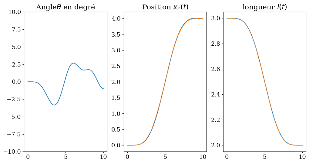
plt.figure(figsize=(12,6))
plt.subplot(1,3,1)
plt.plot(tt,THETA*180/np.pi)
plt.ylim(-10,10)
plt.title("Angle$\\theta$ en degré")
plt.subplot(1,3,2)
plt.plot(tt,XC)
plt.plot(tt,XREF,'--')
plt.title('Position $x_c(t)$')
plt.subplot(1,3,3)
plt.plot(tt,LL)
plt.plot(tt,LREF,'--')
plt.title('longueur $l(t)$')

Text(0.5, 1.0, 'longueur $l(t)$')

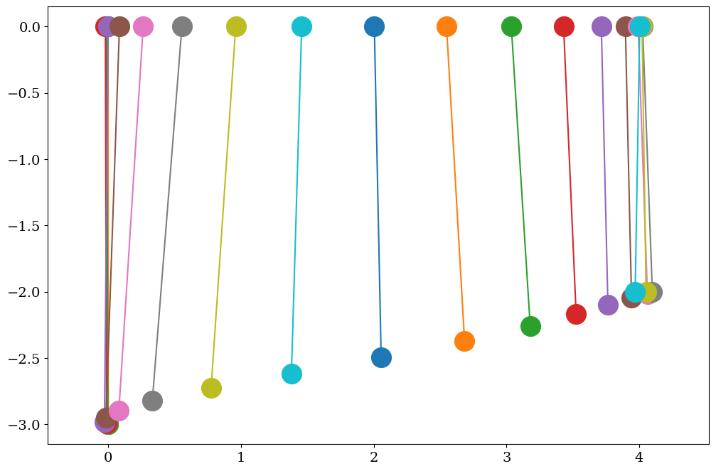
# tracer du mouvement
plt.figure(figsize=(12,8))
for i in range(0,len(tt),20):
    X,Y = [XC[i],XC[i]+LL[i]*np.sin(THETA[i])],[0.,-LL[i]*np.cos(THETA[i])]
    plt.plot(X,Y,'-o',ms=20)
plt.axis('equal')

\[\displaystyle \left( -0.234930948158735, \ 4.30557876347815, \ -3.15, \ 0.15\right)\]

6.6. Evitement d’un obstacle

• au point x=xref/2 on passe au dessus d’un obstacle pour avoir une longueur la < min(l0,lf)

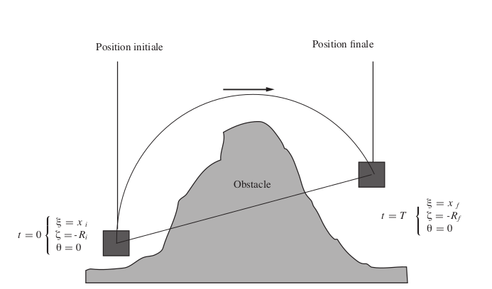
• sans obstacle la trajectoire droite: $\( y = l_0 + (l_f-l_0) x \)$

• avec obstacle tq \(y=y_a\): on xie par une parabole $\( y = l_0 + (l_f-l_0) x (a+bx+cx^2)\)$

avec 3 conditions:

• \(y = l_f\) en x=1

• \(y = l_a\) en x=1/2

• \(\dot{y} = 0\) en x=1/2

pour \(l_a = 2l_f - l_0\) on trouve:

\[ y = l_0 + (l_f-l_0) x (9-12x+4x^2)\]

6.7. FIN