3. Simulation de mouvement en mécanique

Marc BUFFAT, Université Claude Bernard Lyon 1

%matplotlib inline
# bibliotheques de base
import matplotlib
import numpy as np
import matplotlib.pyplot as plt
from matplotlib import rcParams
rcParams['font.family'] = 'serif'
rcParams['font.size'] = 14
from IPython.core.display import HTML

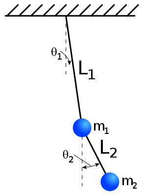
3.1. Mouvement du pendule double

pendule double

3.1.1. expérience: mouvement chaotique

HTML('<iframe width="640" height="360" src="https://www.youtube.com/embed/AwT0k09w-jw" frameborder="0" allowfullscreen></iframe>')

/home/buffat/venvs/jupyter/lib/python3.10/site-packages/IPython/core/display.py:431: UserWarning: Consider using IPython.display.IFrame instead
  warnings.warn("Consider using IPython.display.IFrame instead")

3.1.2. modélisation

import scipy.integrate as integrate
from   time import time

# from http://www.physics.usyd.edu.au/
# modifie par Marc BUFFAT 2014
# parametres
G =  9.8 # acceleration due to gravity, in m/s^2
L1 = 1.0 # length of pendulum 1 in m
L2 = 0.5 # length of pendulum 2 in m
M1 = 1.0 # mass of pendulum 1 in kg
M2 = 1.0 # mass of pendulum 2 in kg

# equation du mvt en theta, dtheta
# U = [theta1, dtheta1, theta2, dtheta2]
def F(U,t):
    """ second membre EDO DU/dt=F(U,t) """
    dydx    = np.zeros((4))
    dydx[0] = U[1]
    delta   = U[2]-U[0]
    den1    = (M1+M2)*L1 - M2*L1*np.cos(delta)*np.cos(delta)
    dydx[1] = (M2*L1*U[1]*U[1]*np.sin(delta)*np.cos(delta)
               + M2*G*np.sin(U[2])*np.cos(delta) + M2*L2*U[3]*U[3]*np.sin(delta)
               - (M1+M2)*G*np.sin(U[0]))/den1
    dydx[2] = U[3]
    den2    = (L2/L1)*den1
    dydx[3] = (-M2*L2*U[3]*U[3]*np.sin(delta)*np.cos(delta)
               + (M1+M2)*G*np.sin(U[0])*np.cos(delta)
               - (M1+M2)*L1*U[1]*U[1]*np.sin(delta)
               - (M1+M2)*G*np.sin(U[2]))/den2
    return dydx

# calcul energie du systeme
def Energie(U):
    Ec1=0.5*M1*(L1*U[1])**2
    Ec2=0.5*M2*((L1*U[1])**2+(L2*U[3])**2
              +2*L1*L2*np.cos(U[2]-U[0])*U[1]*U[3])
    Ep1=-M1*G*L1*np.cos(U[0])
    Ep2=-M2*G*(L2*np.cos(U[2])+L1*np.cos(U[0]))
    H  = Ec1+Ec2+Ep1+Ep2
    return np.array([Ec1,Ec2,Ep1,Ep2,H])

# positions et vitesses initiales
theta1 = np.pi
w1     = -1.5
theta2 = 0.0
w2  = 0.0
# initial state
U0 = np.array([theta1, w1, theta2, w2])
# temps de visualisation
dt = 0.05
tf = 20.0
N  = int(tf/dt)+1;
t  = np.linspace(0.0,tf,N)
#integrate your ODE using scipy.integrate.
debut = time()
y = integrate.odeint(F, U0, t)
cpu = time() - debut
# solution en X,Y
th1 = y[:,0]; th2 = y[:,2]

# tracer
print("Calcul en %.2g sec"%cpu)
print("Energie t=0",Energie(y[0,:]))
print("Energie t=",tf,Energie(y[-1,:]))

Calcul en 0.12 sec
Energie t=0 [ 1.125  1.125  9.8    4.9   16.95 ]
Energie t= 20.0 [13.81088792  7.62023666 -0.52980043 -3.95133817 16.94998599]

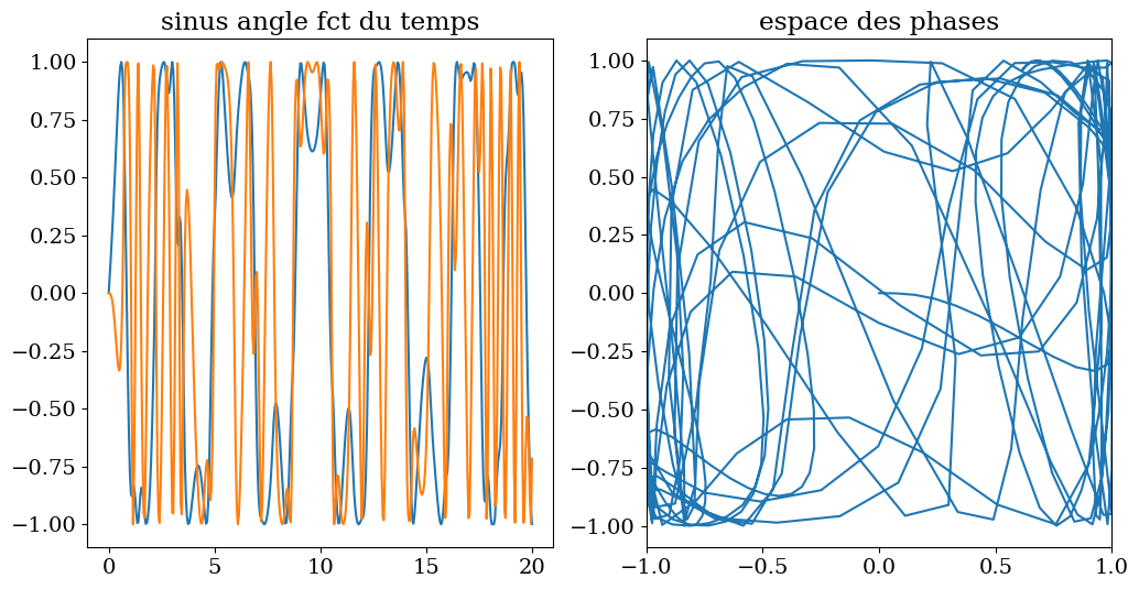
def tracesol(t,th1,th2):
    # tracer solution 
    fig = plt.figure(figsize=(12,6))
    ax1 = fig.add_subplot(121)
    ax1.plot(t,np.sin(th1))
    ax1.plot(t,np.sin(th2))
    ax1.set_title("sinus angle fct du temps")
    ax2 = fig.add_subplot(122)
    ax2.plot(np.sin(th1),np.sin(th2))
    ax2.set_title("espace des phases")
    ax2.axis('equal')
    plt.xlim(-1,1)
    plt.ylim(-1,1)
    return

# tracer solution 
tracesol(t,th1,th2)

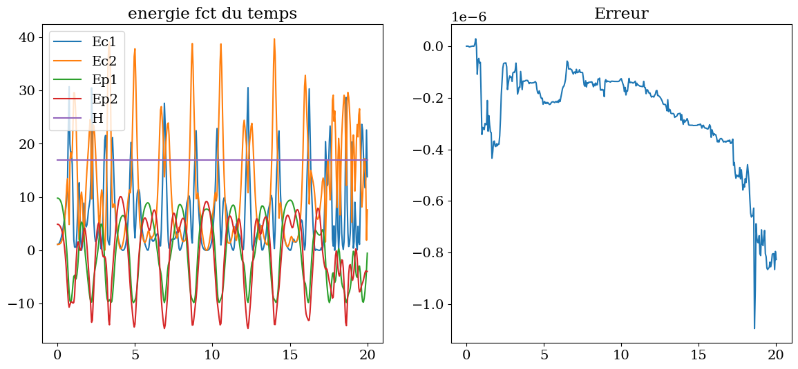
# evolution energie
H=np.zeros((N,5))
for i in range(N):
    H[i,:]=Energie(y[i,:])
# tracer
fig = plt.figure(figsize=(14,6))
ax1 = fig.add_subplot(121)
ax1.plot(t,H[:,0],label="Ec1")
ax1.plot(t,H[:,1],label="Ec2")
ax1.plot(t,H[:,2],label="Ep1")
ax1.plot(t,H[:,3],label="Ep2")
ax1.plot(t,H[:,4],label="H")
ax1.set_title("energie fct du temps")
ax1.legend(loc=0) 
ax2 = fig.add_subplot(122)
ax2.plot(t,(H[:,4]-H[0,4])/H[0,4])
formatter = matplotlib.ticker.ScalarFormatter()
formatter.set_powerlimits((-3,3))
ax2.yaxis.set_major_formatter(formatter)
ax2.set_title("Erreur")

Text(0.5, 1.0, 'Erreur')

# animation 
#from   JSAnimation import IPython_display
import matplotlib.animation as animation
# variables globales
line=None
time_text=None
time_template=None
x1=None; y1=None; x2=None; y2=None;
fig=None; ax1=None

def init():
    global line,time_text
    line.set_data([], [])
    time_text.set_text('')
    return line, time_text,

def animate(i):
    global line,time_text,time_template,x1,x2,y1,y2
    Xp=np.zeros(3); Yp=np.zeros(3);
    Xp[1:] = [x1[i], x2[i]]
    Yp[1:] = [y1[i], y2[i]]
    line.set_data(Xp,Yp)
    time_text.set_text(time_template%(i*dt))
    return line, time_text,

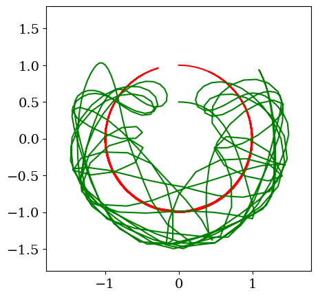
def init_anim(th1,th2):
    global fig,ax1,line,time_text,time_template,x1,y1,x2,y2
    x1 =  L1*np.sin(th1);      
    y1 = -L1*np.cos(th1)
    x2 =  L2*np.sin(th2) + x1; 
    y2 = -L2*np.cos(th2) + y1
    xmin=-1.2*(L1+L2); xmax=-xmin
    ymin=-1.2*(L1+L2); ymax=-ymin
    fig = plt.figure(figsize=(10,5))
    ax1 = fig.add_subplot(111, aspect='equal')
    ax1.set_axis_on()
    ax1.set_xlim((xmin,xmax))
    ax1.set_ylim((ymin,ymax))
    fig.set_facecolor("#ffffff")
    ax1.plot(x1,y1,'-r')
    ax1.plot(x2,y2,'-g')
    line, = ax1.plot([], [], 'o-b', lw=5, markersize=20)
    time_template = 't = %.1fs'
    time_text = ax1.text(0.05, 0.9, '', transform=ax1.transAxes, fontsize=20)
    return

# trace animation
fig = plt.figure(figsize=(14,6))
init_anim(th1,th2)
anim=animation.FuncAnimation(fig, animate,frames= th1.size,
        interval=15, blit=True, init_func=init, repeat = False)

<Figure size 1400x600 with 0 Axes>

HTML(anim.to_html5_video())

3.1.3. modes du pendule double fonction de \(\theta_1\)

# positions et vitesses initiales
w1     = 0.0
theta2 = 0.0
w2     = 0.0
# temps de visualisation
dt = 0.05
tf = 20.0
N  = int(tf/dt)+1;
t  = np.linspace(0.0,tf,N)

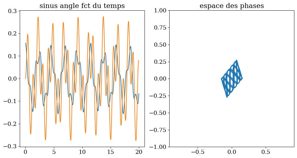
3.1.4. cas lineaire

theta1 = np.pi/20
# cd initiales
U0 = np.array([theta1, w1, theta2, w2])
y = integrate.odeint(F, U0, t)
# solution en X,Y
th1 = y[:,0]; th2 = y[:,2]
tracesol(t,th1,th2)

# trace animation
fig = plt.figure(figsize=(14,6))
init_anim(th1,th2)
anim=animation.FuncAnimation(fig, animate,frames= th1.size,
        interval=15, blit=True, init_func=init, repeat = False)

<Figure size 1400x600 with 0 Axes>

HTML(anim.to_html5_video())

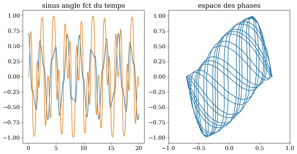
3.1.5. cas non lineaire

theta1 = np.pi/4
# cd initiales
U0 = np.array([theta1, w1, theta2, w2])
y = integrate.odeint(F, U0, t)
# solution en X,Y
th1 = y[:,0]; th2 = y[:,2]
tracesol(t,th1,th2)

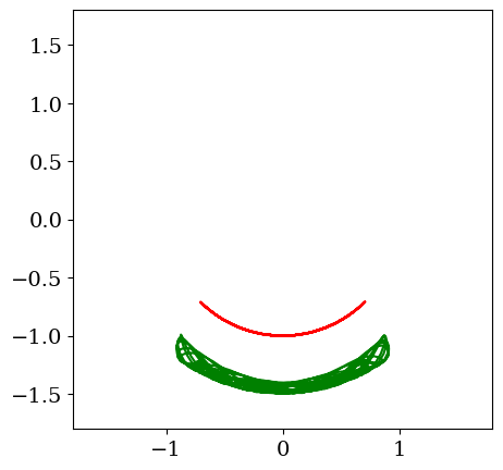
# trace animation
fig = plt.figure(figsize=(14,6))
init_anim(th1,th2)
anim=animation.FuncAnimation(fig, animate,frames= th1.size,
        interval=15, blit=True, init_func=init, repeat = False)

<Figure size 1400x600 with 0 Axes>

HTML(anim.to_html5_video())

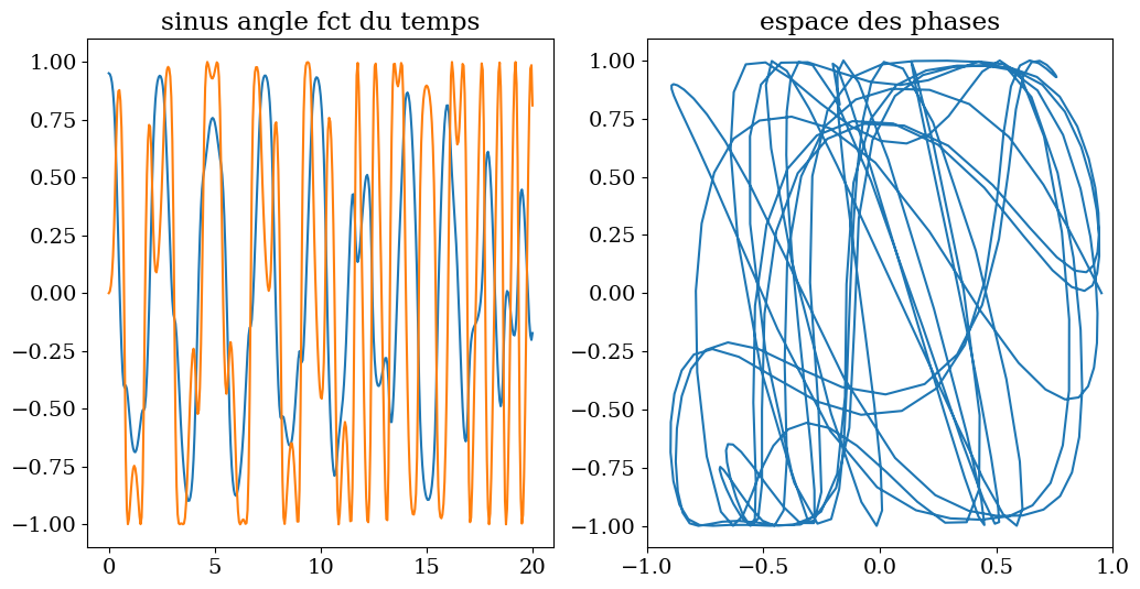
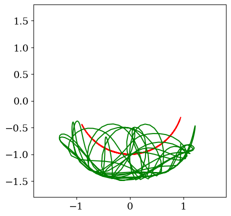
3.1.6. cas chaotique

theta1 = 0.8*np.pi/2
# cd initiales
U0 = np.array([theta1, w1, theta2, w2])
y = integrate.odeint(F, U0, t)
# solution en X,Y
th1 = y[:,0]; th2 = y[:,2]
tracesol(t,th1,th2)

# trace animation
fig = plt.figure(figsize=(14,6))
init_anim(th1,th2)
anim=animation.FuncAnimation(fig, animate,frames= th1.size,
        interval=15, blit=True, init_func=init, repeat = False)

<Figure size 1400x600 with 0 Axes>

HTML(anim.to_html5_video())

3.2. Problème des 3 corps

3.2.1. Modélisation

# Animation problème des 3 corps
# (C) Marc BUFFAT
import matplotlib.pyplot as plt
from matplotlib import animation

# unites astronomiques
Lt =1.49e11 # distance terre soleil
Mt=6.0e24  # masse de la terre
Tt =3600*24*365.25 # annee terrestre
# constante gravitationnelle sans dimension
G=6.67e-11/(Lt**3/Mt/Tt**2)
print("Probleme sans dimension (UAS) G=",G, " avec Tref = 1 annee")
#
# calcul des Forces
# =================
def Force(X):
    """ calcul des forces gravitationnelles / masse """
    Fg=np.zeros(np.shape(X))
    X01=X[1,:]-X[0,:]
    X02=X[2,:]-X[0,:]
    X12=X[2,:]-X[1,:]
    r01 = np.sqrt(np.dot(X01,X01))
    a01 = G*M[0]*M[1]/r01**3
    r02 = np.sqrt(np.dot(X02,X02))
    a02 = G*M[0]*M[2]/r02**3
    r12 = np.sqrt(np.dot(X12,X12))
    a12 = G*M[1]*M[2]/r12**3
    Fg[0,:]=  a01/M[0]*X01 + a02/M[0]*X02
    Fg[1,:]= -a01/M[1]*X01 - a12/M[1]*X12
    Fg[2,:]= -a02/M[2]*X02 + a12/M[2]*X12
    return Fg

Probleme sans dimension (UAS) G= 0.00012048312217859223  avec Tref = 1 annee

# calcul energie du systeme
def Energie(U):
    X01=U[2:4]-U[0:2]
    X02=U[4:6]-U[0:2]
    X12=U[4:6]-U[2:4]
    r01 = np.sqrt(np.dot(X01,X01))
    r02 = np.sqrt(np.dot(X02,X02))
    r12 = np.sqrt(np.dot(X12,X12))
    U0_2 =  np.dot(U[6:8],U[6:8])
    U1_2 =  np.dot(U[8:10],U[8:10])
    U2_2 =  np.dot(U[10:12],U[10:12])
    # par unite de masse
    H0 = 0.5*M[0]*U0_2 - G*( M[0]*M[1]/r01 + M[0]*M[2]/r02)
    H1 = 0.5*M[1]*U1_2 - G*(-M[1]*M[0]/r01 - M[1]*M[2]/r12)
    H2 = 0.5*M[2]*U2_2 - G*(-M[2]*M[0]/r02 + M[2]*M[1]/r12)
    return np.array([H0,H1,H2])

# integration avec ODEint
def F(U,t):
    """ second membre EDO DU/dt=F(U,t) """
    X  = np.reshape(U[0:6],(3,2))
    Fg = Force(X)
    dU = np.zeros(12)
    dU[0:6] = U[6:]
    dU[6: ] = np.reshape(Fg,6)
    return dU

# parametres sans dimension masse, position et vitesse initiale
# soleil
m0 = 1.99e30/Mt
r0 = 0.
# terre
m1 = 1.
r1 = 1.
# jupiter
m2 = 1.9e27/Mt
r2 = 7.75e11/Lt

# calcul des CI (systeme a 2 corps soleil + planete)
# vitesse de rotation du systeme a 2 corps
# terre
R1=r0+r1
omega1=np.sqrt(G*(m0+m1)/(R1**3))
t1=2*np.pi/omega1    # periode
mu1 = m1/(m0+m1)
C1=mu1*R1 # centre de gravite
# Jupiter
R2=r0+r2
omega2=np.sqrt(G*(m0+m2)/(R2**3))
t2=2*np.pi/omega2
mu2 = m2/(m0+m2)
C2=mu2*R2
# d'ou les CI
u1=0.
v1=omega1*(R1-C1)
u2=0.
v2=omega2*(R2-C2)
u0=0.
v0=-omega2*C2 - omega1*C1
rr2 = r2*1.1

3.2.2. utilisation solveur odeint

# cdts initiale: position puis vitesse
M =np.array([m0,m1,m2])
U0=np.array([0., 0.,r1,0,r2,0,u0, v0,u1,v1,u2,v2])
N=500
t = t2  # temps d'integration
T = np.linspace(0,t,N)
debut = time()
U = integrate.odeint(F, U0, T)
cpu = time() - debut
print("position finale :",U[-1,0:6])
print("tcpu odeint :",cpu)

position finale : [ 1.41914415e-06  2.68764184e-06  5.29299130e-01 -8.48970806e-01
  5.20134234e+00 -1.33990745e-04]
tcpu odeint : 0.053229570388793945

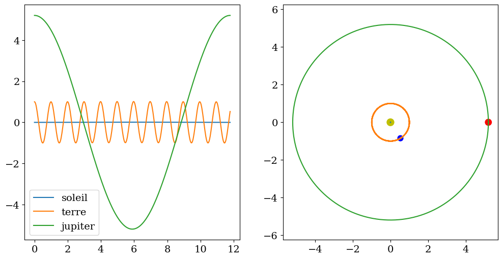
plt.figure(figsize=(12,6))
plt.subplot(1,2,1)
plt.plot(T,U[:,0],label='soleil')
plt.plot(T,U[:,2],label='terre')
plt.plot(T,U[:,4],label='jupiter')
plt.legend(loc=0)
plt.subplot(1,2,2)
plt.axis('equal')
plt.plot(U[:,0],U[:,1])
plt.plot(U[:,2],U[:,3])
plt.plot(U[:,4],U[:,5])
plt.scatter(U[-1,0:6:2],U[-1,1:6:2],c=['y','b','r'],marker='o',s=[100,60,80])

<matplotlib.collections.PathCollection at 0x7f437c0b5030>

# energie
print("Energie t=0",Energie(U[0,:]))
print("Energie t=",tf,Energie(U[-1,:]))
H=np.zeros((N,3))
for i in range(N):
    H[i,:]=Energie(U[i,:])

Energie t=0 [-2471.63103969    59.94937419  3648.102448  ]
Energie t= 20.0 [-2471.62133625    59.92153231  3648.10394574]

plt.figure(figsize=(10,8))
plt.title("Erreur en %")
plt.plot(T,(H[:,0]-H[0,0])/H[0,0],label='soleil')
plt.plot(T,(H[:,1]-H[0,1])/H[0,1],label='terre')
plt.plot(T,(H[:,2]-H[0,2])/H[0,2],label='jupiter')
plt.legend(loc=0)

<matplotlib.legend.Legend at 0x7f437c1460e0>

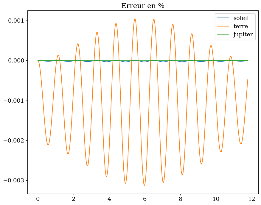
L’erreur est faible, mais peut devenir importante pour des intégrations sur plusieurs milliers d’années. En astro-physique on utilise donc des algorithmes spécifiques conservant l’énergie (mécanique celeste)

solution avec solver implicite BDF (lsoda)

3.3. FIN