3. Planification en Mécanique

Marc BUFFAT dpt mécanique, Université Lyon 1

%matplotlib inline
import numpy as np
import sympy as sp
import matplotlib.pyplot as plt
plt.rc('font', family='serif', size='14')
from IPython.display import display, Markdown, clear_output
def printmd(string):
    display(Markdown(string))
from metakernel import register_ipython_magics
register_ipython_magics()
from sympy.physics.vector import init_vprinting
init_vprinting()

3.1. Modélisation du bras d’une grue à vide (sans charge)

3.2. Calcul symbolique avec sympy (sp)

• variable symbolique: Symbol, symbols

• fonction symbolique: Function

• expression symbolique (variable)

• affichage: display

• transformation en fonction: lambda

• dérivation: diff

• évaluation numerique: evalf, lambdify

• substitution: subs

attention avec Python on utilise des variables symboliques et numériques. Donc attention à ne pas mélanger

• sp.cos() fonction cosinus symbolique

• np.cos() fonction cosinus numérique

3.2.1. Documentation sympy et mechanics

• Sympy: https://docs.sympy.org/latest/index.html

• Mechanics: https://docs.sympy.org/latest/modules/physics/mechanics/index.html

3.3. Problème: modèle de solide en rotation avec 1DDL

• bras en rotation dans le plan

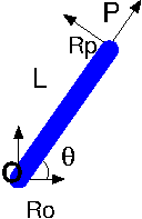
3.4. Modélisation du mouvement d’un solide

1. paramètres et ddl

• définition des parametres avec sp.symbols

• définition des ddl avec dynamicsymbols

2. repère, point

• repère avec ReferenceFrame

• point Point

• definition position des points et repères (rotation)

3. définition des solides

• masse

• matrice d’inertie inertia

4. cinématique / différent repère

• solide indéformable: RigidBody

• vitesse, qte de mouvement linear_momentum angular_momentum

• composition des vitesses v1pt_theory v2pt_theory

5. formalisme lagrangien

• Lagrangian

• Equation de Lagrange

6. résolution numérique

• génération automatique des équations

• changement de variables

• EDO du 1er ordre

3.4.1. paramétrage

• paramètres L, a, (longueur et diamètre du bras), M (masse) , g

• 1 ddl \(\theta\) et \(\dot{\theta}\)

# parametres et ddl
from sympy.physics.mechanics import dynamicsymbols, Point, ReferenceFrame
from sympy.physics.mechanics import RigidBody, Lagrangian, LagrangesMethod
theta   = dynamicsymbols('theta')
thetap  = dynamicsymbols('theta',level=1)
L,a,M,g = sp.symbols('L a M g')
t       = sp.Symbol('t')

3.4.2. repères et position

O = Point('O')
G = Point('G')
P = Point('P')
RO = ReferenceFrame('R_O')
RP = ReferenceFrame('R_P')
# definition position relative P,G et des repères RP,RO
### BEGIN SOLUTION
RP.orient(RO,'Axis',[theta, RO.z])
P.set_pos(O,L*RP.x)
G.set_pos(O,L/2*RP.x)
### END SOLUTION

3.4.3. définition du solide: masse et inertie

from sympy.physics.mechanics import inertia
Ix = M*a**2/2
Iy = M*a**2/4 + M*L**2/12
# definition matrice inertie IG et du solide TigeOP
IG = 0
TigeOP = 0
### BEGIN SOLUTION
IG = inertia(RP,Ix,Iy,Iy)
TigeOP = RigidBody('Tige_OP',G,RP,M,(IG,G))
### END SOLUTION
display("IG:",IG)
display("repère lié au solide:",TigeOP.frame)

'IG:'

'repère lié au solide:'

R_P

3.4.4. cinématique (relation de transport)

O.set_vel(RO,0.)
P.set_vel(RP,0.)
G.set_vel(RP,0.)
# calcul vitesse de P et G avec la relation de transport
### BEGIN SOLUTION
P.v2pt_theory(O,RO,RP)
G.v2pt_theory(O,RO,RP)
### END SOLUTION
display("VP,VG / RO:",P.vel(RO),G.vel(RO))
display("VP,VG / RP:",P.vel(RP),G.vel(RP))

'VP,VG / RO:'

'VP,VG / RP:'

3.4.5. formalisme lagragien (solide indéformable)

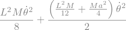
display("mt cinetique, qte mvt, :",TigeOP.angular_momentum(O,RO),TigeOP.linear_momentum(RO))
display("energie cinetique:",TigeOP.kinetic_energy(RO))
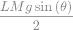
# definition energie potentiel dans TigeOP.potential_energy
### BEGIN SOLUTION
TigeOP.potential_energy = M*g*G.pos_from(O).dot(RO.y)
### END SOLUTION
display("energie potentiel:",TigeOP.potential_energy)

'mt cinetique, qte mvt, :'

'energie cinetique:'

'energie potentiel:'

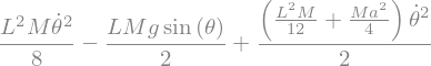
from sympy.physics.mechanics import Lagrangian,LagrangesMethod
# calcul du lagrangien dans La
La = 0
### BEGIN SOLUTION
La=Lagrangian(RO,TigeOP)
### END SOLUTION
display("Lagrangien:",La)

'Lagrangien:'

3.5. Equation de Lagrange

Bilan des forces non conservatives (qui travaillent):

• couple moteur : \(C M\) en O (attention adimensionnalisé par M)

• équation de Lagrange avec LagrangesMethod

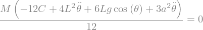
C = sp.symbols('C')
# calcul de l'equation de lagrange dans Eq
Eq = 0
### BEGIN SOLUTION
LM = LagrangesMethod(La,[theta],forcelist=[(RP,C*M*RO.z)],frame=RO)
Eq = LM.form_lagranges_equations()[0]
Eq = Eq.simplify()
### END SOLUTION
display("equation de Lagrange:",sp.Eq(Eq,0))

'equation de Lagrange:'

3.5.1. Mise sous forme matricielle \(A.\dot{Y} = B \)

pour la résolution numérique: transformation en 2 EDO du 1er ordre: $\( \dot{Y} = F(Y) \mbox{ avec } F = A^{-1} B \)$

# calcul de A et B puis F (en simplifiant)
A = 0
B = 0
F = 0
### BEGIN SOLUTION
A=LM.mass_matrix_full
B=LM.forcing_full
display("A=",A,"B=",B)
F = A.inv()*B
F[1]=F[1].simplify()
### END SOLUTION
display('F(Y)=',F)

'A='

'B='

'F(Y)='

3.6. Mouvement oscillant autour position équilibre

\[ \dot{Y} = F(Y) \]

3.6.1. position d’équilibre en \(\theta_0\)

• calcul du couple \(C_0\) assurant l’équilibre

• à partir de l’équation de Lagrange avec \(\ddot{\theta} = 0\)

• utilisation de sp.solve()

# calcul du couple C0 pour un position theta
C0 = 0
### BEGIN SOLUTION
Eq1 = Eq.subs({theta.diff(t,t):0})
display(Eq1)
C0 = sp.solve(Eq1,C)[0]
### END SOLUTION
display("C0=",C0)

'C0='

3.6.2. conversion calcul symbolique -> fonction python

choix des valeurs des paramètres

# fonction FY  avec sp.lambdify
smFY = 0
# parametres
GG = 9.81
LL = 1.0
aa = 0.1
### BEGIN SOLUTION
valnum = [(g,GG), (L,LL), (a,aa)]
smFY = sp.lambdify((theta,thetap,C),F.subs(valnum),'numpy')
### END SOLUTION

# fonction F(Y)
def F(Y,t):
    '''second memebre EDO dY/dt = F(Y)'''
    ### BEGIN SOLUTION
    global CC0
    FF = smFY(Y[0],Y[1],CC0)
    return FF[:,0]
    ### END SOLUTION

# choix du couple C0 pour obtenir une position theta0
# position stable 
Theta0 = -np.pi/4
# position instable
Theta0 =  np.pi/4
# calcul du couple CC0
CC0 = 0
### BEGIN SOLUTION
CC0 = float(C0.subs(theta,Theta0).subs(valnum))
### END SOLUTION
print("Pour theta0={:.3f} C0={:.3f}".format(Theta0,CC0))

Pour theta0=0.785 C0=3.468

3.6.3. simulation numérique

utilisation du solveur odeint

• validation dans le cas theta(0)=theta0

• cas avec perturbation

from scipy.integrate import odeint
# calcul solution THETA et THETAP
### BEGIN SOLUTION
# position d'équilibre
Y0 = np.array([Theta0,0.])
# cas perturbé
Y0 = np.array([Theta0*1.1,0.])
tt  = 1
N   = 200
T = np.linspace(0,tt,N)
sol = odeint(F,Y0,T)
THETA = np.mod(sol[:,0],2*np.pi)
THETAP= sol[:,1]
### END SOLUTION

3.6.4. tracé du résultat

plt.figure(figsize=(10,8))
plt.subplot(2,1,1)
plt.title('trajectoire non controllée')
plt.plot(T,THETA,label="$\\theta(t)$")
plt.plot(T,Theta0*np.ones(THETA.size),'--',label="$\\theta_0$")
plt.legend()
plt.xlabel('t')
plt.subplot(2,1,2)
plt.plot(LL*np.cos(THETA),LL*np.sin(THETA),'-')
plt.plot([LL*np.cos(Theta0)],[LL*np.sin(Theta0)],'*',ms=12)
plt.plot([LL*np.cos(THETA[0])],[LL*np.sin(THETA[0])],'o',ms=12)
plt.plot([0,LL*np.cos(Theta0)],[0,LL*np.sin(Theta0)],'--')
plt.xlabel('$X_P$')
plt.ylabel('$Y_P$')
plt.axis('equal');

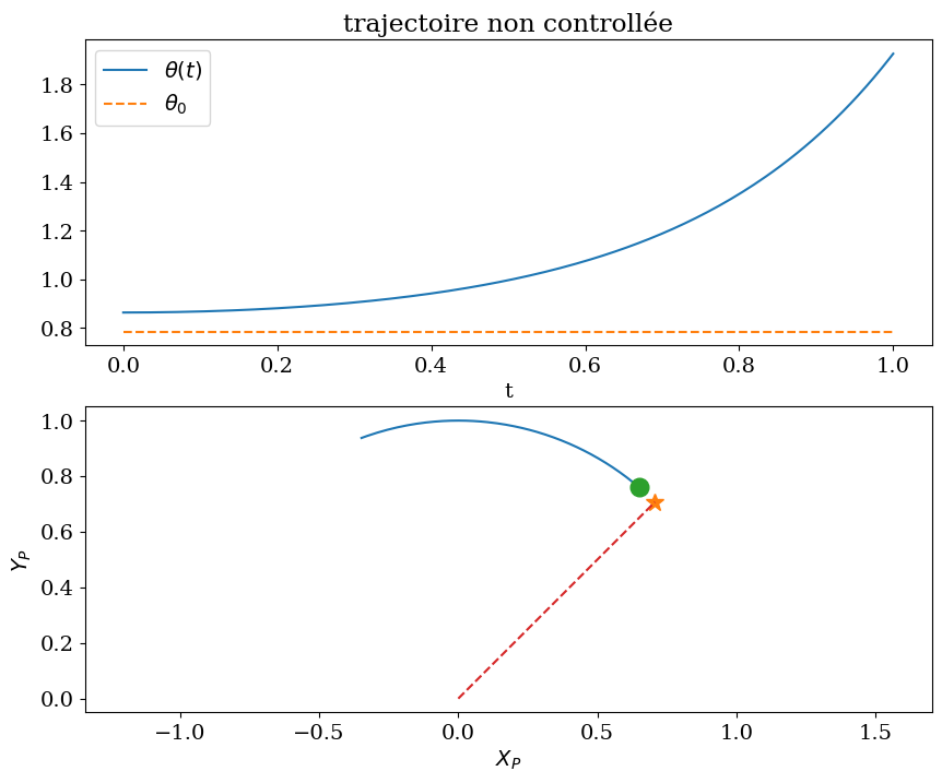
3.6.5. analyse

• pour \(\theta_0 > 0\) : position instable !!!

• pour \(\theta_0 < 0\) : position stable !!!

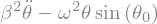
paramétrisation de l’équation en fonction de \(\omega\) \(\beta\)

• \(\omega =\sqrt{\frac{g}{L}}\)

• \(\beta^2 \) coefficient de \(\ddot{\theta}\)

\[ \beta^2 = \frac{a^2}{2L^2} + \frac{2}{3} \]

display("Equation:",sp.Eq(2*Eq/(L**2*M),0))
omega, beta, theta0 = sp.symbols('omega beta theta_0')

'Equation:'

rels = 0
eq1 = 0
### BEGIN SOLUTION
rels = [(g,omega**2*L),(a**2,(beta**2-2/3)*2*L**2)]
Eq1 = 2*Eq/(L**2*M)
Eq1 = Eq1.subs(rels).simplify()
### END SOLUTION
display(Eq1)

# equation à l'équilibre -> theta0
Eq0 = 0
### BEGIN SOLUTION
Eq0=Eq1.subs({theta.diff(t,t,):0,theta:theta0})
display(Eq0)
### END SOLUTION
# equation fct de theta0
Eq0=Eq1-Eq0
display(sp.Eq(Eq0,0))

### linéarisation autour de la position d’équilibre \(\theta_0\)

\[\theta = \theta_0+\theta' \mbox{ avec } \theta' \ll 1\]

# linearisation autour de theta0, en remplacant theta par theta+theta0
Eq1 = 0
### BEGIN SOLUTION
Eq1 = Eq0.subs({theta:theta+theta0})
display(Eq1)
Eq1 = Eq1.subs({sp.cos(theta0+theta):sp.cos(theta0)-sp.sin(theta0)*theta})
Eq1 = Eq1.simplify()
### END SOLUTION
display("linéarisation ",Eq1)

'linéarisation '

3.6.6. Analyse de solution linéarisée

• stabilité si \(\sin(\theta_0) < 0\)

• si on impose un couple \(C_0\) correspondant à l’équilibre quasi-statique $\( C_0 = \frac{L g \cos\theta}{2} = \frac{\omega^2 L^2 \cos\theta}{2}\)\( possibilité d'instabilité: \)\(\ddot{\theta} \approx 0\)$

• dans le cas instable nécessité d’un feedback (contrôle) p.e. $\( C = C_0 - \alpha (\theta-\theta_0) \)$

3.7. Mouvement imposé du bras

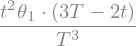
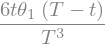
On étudie le positionnement du bras de \(\theta_0=0\) à \(\theta_1\) pendant un temps \(T_0\) en imposant la cinématique

3.7.1. cinématique imposée \(\Theta(t)\)

• conditions $\(\Theta(0)=0, \dot{\Theta}(0)=0, \Theta(T)=\theta_1, \dot{\Theta}(T)=0\)$

• cinématique

\[\Theta(t) = \frac{\theta_1 t^2(3T-2t)}{T^3} \]

• calcul du couple C

# cinematique imposée
t = sp.symbols('t')
theta1,T = sp.symbols('theta_1 T')
Theta = sp.lambdify(t,theta1*t**2*(3*T-2*t)/T**3,'numpy')
display("loi Theta(t):",Theta(t))
display("dérivee:",sp.diff(Theta(t),t).simplify())

'loi Theta(t):'

'dérivee:'

3.7.2. simulation : calcul du couple CC

solution analytique en imposant \(\theta = \Theta(t)\) imposé

from sympy.solvers import solve
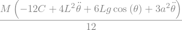
# calcul du couple analytiquement en remplacant dans l'equation linearisée
display(Eq)
### BEGIN SOLUTION
Eq1=Eq.subs({theta:Theta(t),theta.diff(t,t):Theta(t).diff(t,t)})
display(Eq1)
CC=solve(Eq1,C)[0].simplify()
### END SOLUTION
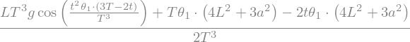
display("C=",CC)

'C='

# conversion en fonction numpy CClin
CClin = sp.lambdify((t,T,theta1),CC.subs(valnum),'numpy')

TT = 2.
Theta1 = np.pi/4
tt = np.linspace(0,TT,100)
# solution linearisée
cc = CClin(tt,TT,Theta1)
plt.plot(tt,cc)
plt.xlabel('t')
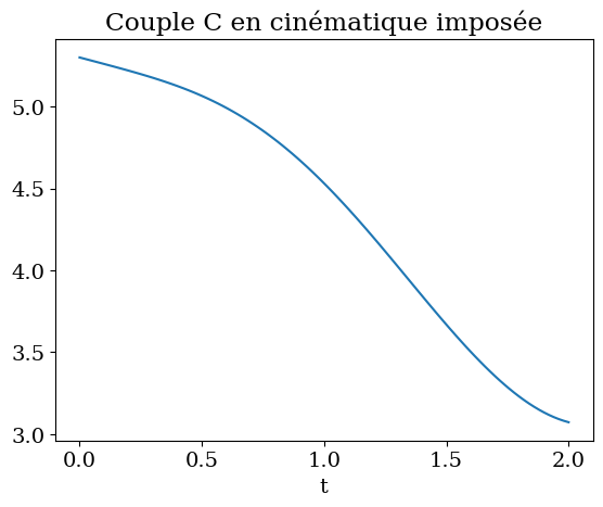
plt.title('Couple C en cinématique imposée');

3.7.3. simulation du pble

résolution EDO avec C donnée par CClin

# fonction F(Y)
def F(Y,t):
    '''second membre de dY/dt = F(Y)  avec Y=[theta, thetap]'''
    global TT,Theta1
    ### BEGIN SOLUTION
    CC = CClin(t,TT,Theta1)
    FF =smFY(Y[0],Y[1],CC)
    return FF[:,0]
    ### END SOLUTION

# simulation 
Y0 = np.array([0.,0.])
# cas avec une perturbation initiale: pble !
#Y0 = np.array([0.1,0.])
#
N   = 200
tt = np.linspace(0,TT,N)
sol = odeint(F,Y0,tt)
THETA = np.mod(sol[:,0],2*np.pi)
THETAP= sol[:,1]
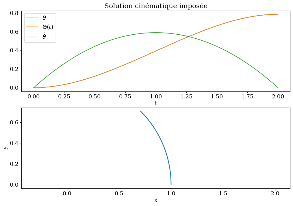
# solution imposée
THETA1=sp.lambdify([t],Theta(t).subs({T:TT,theta1:Theta1}),'numpy')

# tracer de la solution
plt.figure(figsize=(12,8))
plt.subplot(2,1,1)
plt.title('Solution cinématique imposée')
plt.plot(tt,THETA,label="$\\theta$")
plt.plot(tt,THETA1(tt),label="$\\Theta(t)$")
plt.plot(tt,THETAP,label="$\dot{\\theta}$")
plt.legend()
plt.xlabel('t')
plt.subplot(2,1,2)
plt.plot(LL*np.cos(THETA),LL*np.sin(THETA),'-',lw=2)
plt.xlabel('x')
plt.ylabel('y')
plt.axis('equal');

3.8. Modèle dynamique

On souhaite introduire un contrôle dynamique de la commande

On veut définir la commande \(C\) (i.e. le couple) dans l’équation du mouvement: $\( \mathbf{I} \ddot{\theta} = \mathbf{M} C + F(\theta,\dot{\theta})\)\( tel que le mouvement de \)\theta_0\( à \)\theta_1$ soit le plus régulier possible.

Pour cela on va calculer \(C\) en fonction d’un contrôle \(u(t)\). On choisit le couple \(C\) par une opération de découplage et feedback en fonction d’un contrôle \(u\) t.q. $\( \mathbf{M} C = \mathbf{I} u - F(\theta_u,\dot{\theta_u})\)\( ce qui conduit à un système d'EDO linéaires indépendantes (\)u\( étant fixé) \)\( \mathbf{I}\ddot{\theta_u} = \mathbf{I} u \mbox{ soit } \ddot{\theta_u} = u \)$

démarche

1. on choisit la forme du contrôle \(u(t)\) en fonction de \(\theta_u\) et \(\dot{\theta_u}\),

2. à partir de la solution \(\theta_u\) de EDO linéaire \(\ddot{\theta_u} = u\) on définit les parametres du contrôle tq \(\theta_u \approx \theta_{opt}\)

3. on en déduit la commande \(C\) t.q.
   $\( \mathbf{M} C = \mathbf{I} u - F(\theta,\dot{\theta})\)$

4. connaissant \(C\) on peut alors résoudre le problème sous contrôle:

\[ \mathbf{I} \ddot{\theta} = \mathbf{M} C + F(\theta,\dot{\theta})\]

3.8.1. définition de commande \(u\)

On veut positionner le bras avec un angle \(\theta_1\) (et arrivant avec une vitesse nulle).

On part d’une position \(\theta_0=0\) avec une vitesse nulle.

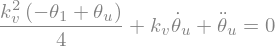
On applique donc une commande \(\mathbf{u}\) proportionnelle à l’écart \(\theta-\theta_1\) et à sa dérivée \(\dot{\theta}\) (feedback): $\( \mathbf{u} = -k_p (\theta-\theta_1) - k_v \dot{\theta} \)\( L'équation du mouvement se réduit à : \)\( \ddot{\theta} + k_v \dot{\theta} + k_p (\theta-\theta_1) = 0 \)$

On choisit les constantes \(k_p\) et \(k_v\) de façon à être dans le régime critique, i.e. avoir un retour à la position le plus rapidement possible sans oscillation. Le discrimant de l’équation caractéristique est alors nul $\( \Delta = k_v^2 - 4 k_p = 0 \mbox{ soit } k_p = k_v^2/4 \)$

les conditions initiales sont la position \(\theta_0=0\) avec une vitesse initiale nulle $\( \theta(0) = 0 \mbox{ et } \dot{\theta}(0) = 0 \)\( La valeur de \)k_v\( fixe le temps de parcours de la trajectoire \)T\( \)\( \theta(T) \approx \theta_1\)\( soit pour une précision relative \)\epsilon\( \)\( k_v \approx - \frac{2}{T} \log \epsilon \)$

# calcul de la solution theta_u avec dsolve
theta_u = sp.Function('theta_u')
kv = sp.symbols('k_v',positive=True)
# ecrire l'équation sur theta_u et en déduire sa solution theta_s avec dsolve
eq = 0
theta_s = 0
### BEGIN SOLUTION
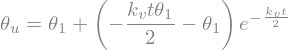
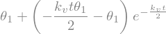
eq = sp.Eq(sp.Derivative(theta_u(t),t,t) + kv*sp.Derivative(theta_u(t),t) + kv*kv/4*(theta_u(t)-theta1) , 0 )
display("equation sur theta_u",eq)
solq=sp.dsolve(eq, theta_u(t), ics={theta_u(0):0, theta_u(t).diff(t).subs(t,0):0})
display("solution",solq)
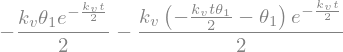
theta_s=sp.Lambda(t,solq.rhs)
display("theta_s(t)",theta_s(t))
### END SOLUTION

'equation sur theta_u'

'solution'

'theta_s(t)'

from sympy.plotting import plot
# parametres
Eps = 1.e-3
Kv  = float((-2/TT)*np.log(Eps))
# vérification et tracer de la solution 
cdtsu = [(theta1,Theta1),(kv,Kv),(T,TT)]
### BEGIN SOLUTION
display("theta_s(T):",theta_s(T))
print("theta_s(T)={:.3f} Theta1={:.3f}".format(theta_s(T).subs(cdtsu),Theta1))
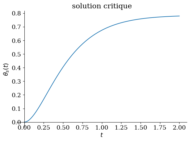
plot(theta_s(t).subs(cdtsu),(t,0,TT), ylabel='$\\theta_s(t)$',title='solution critique');
### END SOLUTION

'theta_s(T):'

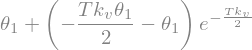
theta_s(T)=0.779 Theta1=0.785

3.8.2. calcul du contrôle pour la trajectoire choisie

• \(\theta\) doit varier de \(\theta_0\) à \(\theta_1\)

• on impose la solution calculée \(\theta_s\) et sa dérivée et on en déduit le contrôle

# solution imposée theta_s
display("theta_s(t):",theta_s(t))
display("dtheta_s  :",theta_s(t).diff(t))
# conversion en fonction python
Theta_s  = 0
dTheta_s = 0
### BEGIN SOLUTION
Theta_s  = sp.lambdify(t,theta_s(t).subs(cdtsu))
dTheta_s = sp.lambdify(t,theta_s(t).diff(t).subs(cdtsu))
### END SOLUTION

'theta_s(t):'

'dtheta_s  :'

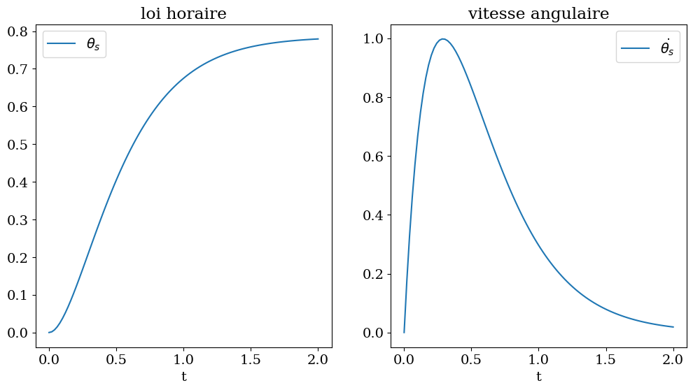
tt = np.linspace(0,TT,100)
fig,(ax1,ax2) = plt.subplots(1,2,figsize=(12,6))
ax1.plot(tt,Theta_s(tt),label="$\\theta_s$")
ax1.set_title("loi horaire")
ax1.set_xlabel('t')
ax1.legend()
ax2.plot(tt,dTheta_s(tt),label="$\\dot{\\theta_s}$")
ax2.set_title("vitesse angulaire")
ax2.set_xlabel('t')
ax2.legend();

3.8.2.1. contrôle \(u_s(t)\)

• feedback $\( \mathbf{u_s} = -k_p (\theta(t)-\theta_1(T)) - k_v \dot{\theta}(t) \)$

avec \(k_p = kv^2/4 \)

# calcul de u_s
u_s = 0
### BEGIN SOLUTION
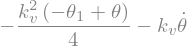
u_s = -kv*sp.diff(theta,t) - kv*kv/4*(theta-theta1)
### END SOLUTION
display("u_s(t):",u_s)

'u_s(t):'

3.8.2.2. couple \(C\)

connaissant \(\theta_u\) et \(u\), on calcul \(C\) t.q.: $\( \mathbf{M} C = \mathbf{I} u - F(\theta,\dot{\theta})\)$

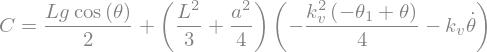
CC = (L**2/3+a**2/4)*u_s + L*g*sp.cos(theta)/2
sp.Eq(C,CC)

# conversion en fonction Python Cs
Cs = sp.lambdify([theta,thetap],CC.subs(cdtsu).subs(valnum),'numpy')

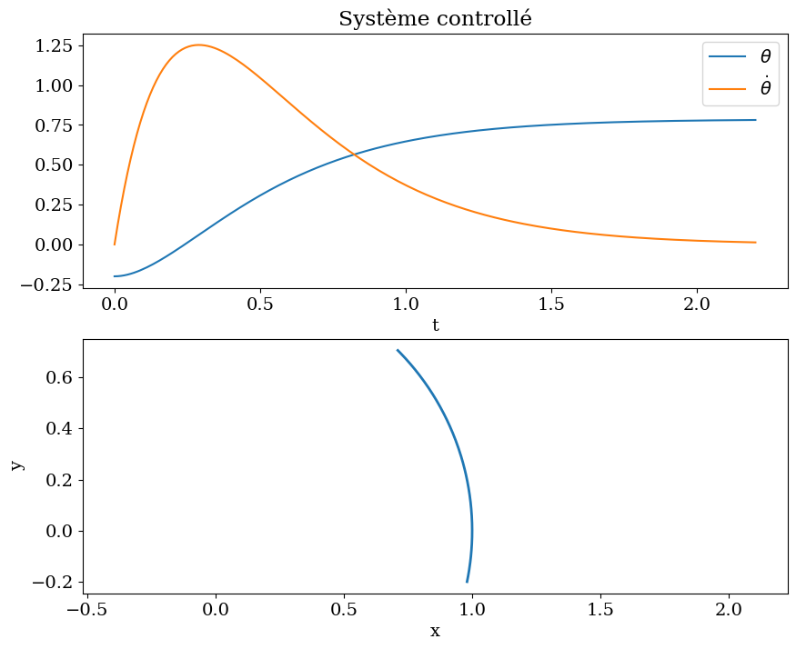
3.8.3. simulation du système controlé

# fonction F(Y)
def F(Y,t):
    '''second membre de dY/dt = F(Y)  avec Y=[theta, thetap]'''
    ### BEGIN SOLUTION
    CC = Cs(Y[0],Y[1])
    FF =smFY(Y[0],Y[1],CC)
    return FF[:,0]
    ### END SOLUTION

# simulation système controle
Y0 = np.array([0.,0.])
# cas avec une perturbation
Y0 = np.array([-0.2,0.])
#
N  = 200
tt = np.linspace(0,TT*1.1,N)
sol = odeint(F,Y0,tt)
THETA = sol[:,0]
THETAP= sol[:,1]

plt.figure(figsize=(10,8))
plt.subplot(2,1,1)
plt.title("Système controllé")
plt.plot(tt,THETA,label="$\\theta$")
plt.plot(tt,THETAP,label="$\dot{\\theta}$")
plt.legend()
plt.xlabel('t')
plt.subplot(2,1,2)
plt.plot(LL*np.cos(THETA),LL*np.sin(THETA),'-',lw=2)
plt.xlabel('x')
plt.ylabel('y')
plt.axis('equal');

3.9. FIN de la leçon