2. Calcul symbolique avec Python/Sympy

Marc BUFFAT, dpt mécanique, Université Claude Bernard Lyon 1

Mise à disposition selon les termes de la Licence Creative Commons
Attribution - Pas d’Utilisation Commerciale - Partage dans les Mêmes Conditions 2.0 France.

Some Tex macros & lib $\(\newcommand{\dt}[1] {\frac{d{#1}}{dt}}\)$

# bibliothéque python
%matplotlib inline
import numpy as np
import sympy as sp
import matplotlib.pyplot as plt
from IPython.core.display import HTML
from IPython.display import display,Image
from sympy.physics.vector import init_vprinting
init_vprinting(use_latex='mathjax', pretty_print=False)

2.1. Calcul symbolique avec sympy (sp)

• variable symbolique: Symbol, symbols

• fonction symbolique: Function

• expression symbolique (variable)

• affichage: display

• transformation en fonction: lambda

• derivation: diff

• evaluation numerique: evalf, lambdify

• substitution: subs

# symbols
t , a ,omega = sp.symbols('t a omega')
V = sp.Function('V')
display(V(0),V(t+1),omega*t/a)

\[\displaystyle V{\left(0 \right)}\]

\[\displaystyle V{\left(t + 1 \right)}\]

\[\displaystyle \frac{\omega t}{a}\]

# expression
Exp = a*sp.sin(omega*t+2)
display(Exp)

\[\displaystyle a \sin{\left(\omega t + 2 \right)}\]

# expression symbolique = arbre
def render_sympy_tree(expr):
    """Render the given Sympy Expression as a graphical tree, inside an IPython notebook"""
    from sympy.printing.dot import dotprint
    import tempfile
    import subprocess
    import os
    from IPython.display import SVG 
    with tempfile.NamedTemporaryFile(mode='w', delete=False) as out_fh:
        out_fh.write(dotprint(expr))
    subprocess.run(['/usr/bin/dot', '-Tsvg', out_fh.name, '-o', out_fh.name + ".svg"])
    svg = SVG(filename=(out_fh.name + ".svg"))
    os.unlink(out_fh.name)
    os.unlink(out_fh.name + ".svg")
    return svg
display(sp.srepr(Exp))
svg=render_sympy_tree(Exp)
display(svg)

"Mul(Symbol('a'), sin(Add(Mul(Symbol('omega'), Symbol('t')), Integer(2))))"

# fonction / derivation
display("Exp=",Exp)
U = lambda t:Exp
display(sp.diff(U(t),t))
display(sp.diff(Exp,t,t))

'Exp='

\[\displaystyle a \sin{\left(\omega t + 2 \right)}\]

\[\displaystyle a \omega \cos{\left(\omega t + 2 \right)}\]

\[\displaystyle - a \omega^{2} \sin{\left(\omega t + 2 \right)}\]

# evaluation python
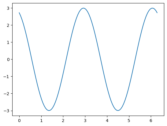
display(Exp.subs({omega:2,a:3}))
UU = sp.lambdify(t,Exp.subs({omega:2.0,a:3}))
TT = np.linspace(0,2*np.pi,100)
YY = UU(TT)
plt.plot(TT,YY)

\[\displaystyle 3 \sin{\left(2 t + 2 \right)}\]

[<matplotlib.lines.Line2D at 0x7f2407d082e0>]

2.2. Mécanique des systèmes indéformables

(C) Rubrique à brac (Gotlib)

mécanique: étude générale du mouvement des systèmes physiques

• cinématique: (du grec kinêma, le mouvement) est l’étude des mouvements indépendamment des causes qui les produisent, ou, plus exactement, l’étude de tous les mouvements possibles.

• dynamique: (du grec dynamikos, puissant, efficace) est une discipline de la mécanique classique qui étudie les corps en mouvement sous l’influence des actions mécaniques qui leur sont appliquées.

Utilisation de la formulation Lagrangienne en mécanique.

2.3. Modèles mécaniques indéformables

\(R_0\) référentiel fixe

point matériel définit par :

• sa position \(P /R_0\) et sa masse \(m\).

solide indéformable définit par

• la position \(G /R_0\) du centre de masse, sa masse \(M\),

• ses rotations \(\Theta\) par rapport à \(/R_0\) autour du centre de gravité \(G\), et sa matrice d’inertie \(I_G\) en \(G\) \(/R_0\).

dégrés de liberté (DOF) paramêtres indépendants du mouvement

• déplacement (translation): maximum 3 (coordonnées du point ou du centre de gravité)

• rotation autour d’un point: maximum 3 (rotation ou angles d’Euler)

• point matériel: 3 DDL max

• solide indéformable: 6 DDL max

2.4. Référentiels: position et dérivation

• \(R_O\) référentiel fixe (orthonormée), repère mobile \(R_P\)

\[ \vec{OM} = x \vec{R}_{O_x} + y \vec{R}_{O_y} + z \vec{R}_{O_z}\]

\[ \vec{OM} = x_1 \vec{R}_{P_x} + y_1 \vec{R}_{P_y} + z_1 \vec{R}_{P_z}\]

• dérivation / repère fixe \(R_O\)

\[ \dt{\vec{OM}} = \dt{x} \vec{R}_{O_x} + \dt{y} \vec{R}_{O_y} + \dt{z} \vec{R}_{O_z}\]

• dérivation / repère mobile \(R_P\)

\[ \dt{\vec{OM}}|R_P = \dt{x_1} \vec{R}_{P_x} + \dt{y_1} \vec{R}_{P_y} + \dt{z_1} \vec{R}_{P_z}\]

\[ \dt{\vec{OM}}|R_O = \dt{\vec{OM}}|R_P + x_1\dt{\vec{R}_{P_x}} + y_1\dt{\vec{R}_{P_y}} + z_1\dt{\vec{R}_{P_z}}\]

• \(\mathcal R\) matrice de rotation de \(R_P\) / \(R_O\), vecteur rotation \(\Omega_{R_P}\) $\( \dt{\vec{R}_{P_x}} = \mathcal{R} \vec{R}_{P_x} = \vec{\Omega}_{R_P}\wedge\vec{R}_{P_x}\)$

• loi de composition des vitesses entre 2 points A et B (et des accélérations)

  • v1pt_theory: A et B quelconques $\( \vec{V}_B | R_O = \vec{V}_A | R_O + \vec{V}_B | R_P + \Omega R_P|R_O \wedge \vec{AB} \)$

  • v2pt_theory: A et B appartiennent au même solide \(R_P\) ( \(\vec{\Omega}\) (taux de rotation de \(R_P\) / \(R_O\)))

\[ \vec{V}_B | R_O = \vec{V}_A | R_O + \vec{\Omega} \wedge \vec{AB} \]

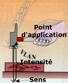
2.5. Equations de Lagrange

• principe des travaux virtuels

• définition du Lagrangien $\( L(q_i) = T(q_i,\dot{q}_i)-U(q_i) \)$

• bilan des travaux virtuels avec des forces généralisées \(F_i\) $\( \sum \frac{d}{dt}(\frac{\partial L}{\partial \dot{q}_i}) \delta q_i - \sum \frac{\partial L}{\partial q_i} \delta q_i = \sum F_i \delta q_i \)$

• équations de Lagrange $\( \frac{d}{dt}(\frac{\partial L}{\partial \dot{q}_i})-\frac{\partial L}{\partial q_i} = F_i \)$

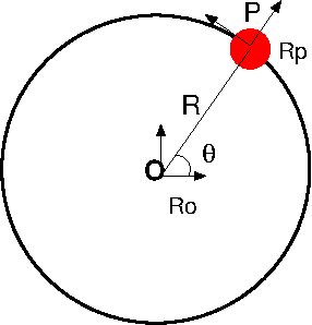
2.6. Masse m sur un cercle de rayon \(R\)

• question: analyse du problème (Point matériel)

2.6.1. modélisation sympy

• utilisation bibliothèque Classical Mechanics

• sympy.physics.mechanics

• Point, ReferenceFrame

• ddl dynamicsymbols

2.6.2. paramètres et DDL

Mouvement plan avec un seul degré de liberté \(\theta(t)\)

• degré de liberté: \(\theta(t)\)

• paramètres du problème

from sympy.physics.mechanics import dynamicsymbols, Point, ReferenceFrame
theta = dynamicsymbols('theta')
R,m,g = sp.symbols('R m g')
print(theta,R)
display(theta*R)

theta(t) R

\[\displaystyle R \theta\]

2.6.3. Référentiel et point

• fonctions ReferenceFrame et Point

• \(R_O\) repère de base et \(R_P\) repère lié au point

• definit les points

• affiche les coordonnées dans un repère dcm matrice de passage de \(R_O\) dans \(R_P\) (direction cosinus matrix)

O = Point('O')
RO = ReferenceFrame('R_O')
P = Point('P')
RP = ReferenceFrame('R_P')
RP.orient(RO,'Axis',[theta, RO.z])
P.set_pos(O,R*RP.x)
P.pos_from(O),P.pos_from(O).express(RO)

\[\displaystyle \left( R\mathbf{\hat{r_p}_x}, \ R \cos{\left(\theta \right)}\mathbf{\hat{r_o}_x} + R \sin{\left(\theta \right)}\mathbf{\hat{r_o}_y}\right)\]

2.6.4. cinématique

• on spécifie la vitesse de O et la vitesse P dans \(R_P\)

• utilisation de la fonction v1pt_theory

O.set_vel(RO,0.)
P.set_vel(RP,0.)
P.v1pt_theory(O,RO,RP)
VP = P.vel(RO)
VP,VP.express(RO),O.vel(RO) + P.vel(RP) + RP.ang_vel_in(RO).cross(P.pos_from(O))

\[\displaystyle \left( R \dot{\theta}\mathbf{\hat{r_p}_y}, \ - R \sin{\left(\theta \right)} \dot{\theta}\mathbf{\hat{r_o}_x} + R \cos{\left(\theta \right)} \dot{\theta}\mathbf{\hat{r_o}_y}, \ R \dot{\theta}\mathbf{\hat{r_p}_y}\right)\]

2.6.5. accélération

• calcul accélération de \(P\) dans \(R_O\)

• formule de composition des accélérations $\( \vec{\Gamma}_P | R_O = \vec{\Gamma}_P| R_P + \vec{\Gamma}_O| R_O + \frac{d}{dt}(\vec{\Omega}_{R_P}) \wedge \vec{OP} + \vec{\Omega}_{R_P}\wedge\vec{\Omega}_{R_P}\wedge\vec{OP} + 2 \vec{\Omega}_{R_P} \wedge \vec{V_P}|R_P \)$

• utilisation de a1pt_theory

P.a1pt_theory(O,RO,RP)
GP = P.acc(RO)
GP, GP.express(RO)

\[\displaystyle \left( - R \dot{\theta}^{2}\mathbf{\hat{r_p}_x} + R \ddot{\theta}\mathbf{\hat{r_p}_y}, \ (- R \sin{\left(\theta \right)} \ddot{\theta} - R \cos{\left(\theta \right)} \dot{\theta}^{2})\mathbf{\hat{r_o}_x} + (- R \sin{\left(\theta \right)} \dot{\theta}^{2} + R \cos{\left(\theta \right)} \ddot{\theta})\mathbf{\hat{r_o}_y}\right)\]

2.6.6. bilan des forces

• question: analyse des forces

2.6.7. formalisme lagrangien

définition d’une particule Par de position \(P\) et de masse \(m\)

#  point materiel = particule masse m
from sympy.physics.mechanics import Particle
Pa = Particle('Pa',P,m)
display(Pa.point.vel(RO),Pa.kinetic_energy(RO))

\[\displaystyle R \dot{\theta}\mathbf{\hat{r_p}_y}\]

\[\displaystyle \frac{R^{2} m \dot{\theta}^{2}}{2}\]

# energie potentiel
Pa.potential_energy = m*g*Pa.point.pos_from(O).dot(RO.y)
Pa.potential_energy

\[\displaystyle R g m \sin{\left(\theta \right)}\]

# lagrangien
from sympy.physics.mechanics import Lagrangian, LagrangesMethod
LPa = Lagrangian(RO,Pa)
display(LPa)

\[\displaystyle \frac{R^{2} m \dot{\theta}^{2}}{2} - R g m \sin{\left(\theta \right)}\]

# equations de lagrange
LMa = LagrangesMethod(LPa,[theta])
LMa.form_lagranges_equations()

\[\displaystyle \left[\begin{matrix}R^{2} m \ddot{\theta} + R g m \cos{\left(\theta \right)}\end{matrix}\right]\]

2.7. Solide en rotation / a O

• barre en rotation autour de O

• question: analyse du problème

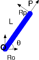
2.7.1. repère et point

• repere fixe \(R_O\), lié au solide \(R_P\)

• points O, P et G

• paramètres L et DDL \(\theta\)

theta = dynamicsymbols('theta')
L     = sp.symbols('L')
O = Point('O')
RO = ReferenceFrame('R_O')
P = Point('P')
RP = ReferenceFrame('R_P')
RP.orient(RO,'Axis',[theta, RO.z])
P.set_pos(O,L*RP.x)
G = Point('G')
G.set_pos(O,L/2*RP.x)

2.7.2. masse / inertie d’un solide

la tige \(OP\) est un solide (cylindre homogène):

• de longueur \(L\) et de rayon \(a\), de masse \(M\)

• de centre de gravité \(G\) tq \(\vec{OG} = \frac{1}{2} \vec{OP}\)

• de matrice d’inertie en \(G\) dans \(R_P\)

\[\begin{split}I(G,R_P) = \begin{pmatrix} I_{x} & 0 & 0 \\ 0 & I_{y} & 0 \\ 0 & 0 & I_{y} \end{pmatrix}\end{split}\]

  - avec $I_{x} = \frac{1}{2} M a^2 $ et $I_{y} = \frac{1}{4} M a^2 + \frac{1}{12} M L^2$

from sympy.physics.mechanics import inertia
a,M,g = sp.symbols('a M g')
Ix = M*a**2/2
Iy = M*a**2/4 + M*L**2/12
IG = inertia(RP,Ix,Iy,Iy)
display(IG)

\[\displaystyle \frac{M a^{2}}{2}\mathbf{\hat{r_p}_x}\otimes \mathbf{\hat{r_p}_x} + (\frac{L^{2} M}{12} + \frac{M a^{2}}{4})\mathbf{\hat{r_p}_y}\otimes \mathbf{\hat{r_p}_y} + (\frac{L^{2} M}{12} + \frac{M a^{2}}{4})\mathbf{\hat{r_p}_z}\otimes \mathbf{\hat{r_p}_z}\]

2.7.3. vitesse

• utilisation de la composition des vitesses: O,G et P appartiennent au même solide

• fonction v2pt_theory

O.set_vel(RO,0.)
P.v2pt_theory(O,RO,RP)
G.v2pt_theory(O,RO,RP)
P.vel(RO),G.vel(RO)

\[\displaystyle \left( L \dot{\theta}\mathbf{\hat{r_p}_y}, \ \frac{L \dot{\theta}}{2}\mathbf{\hat{r_p}_y}\right)\]

2.7.4. Bilan des forces

• question: analyse des forces

2.7.5. définition solide indéformable

• RigidBody

from sympy.physics.mechanics import Lagrangian, RigidBody, LagrangesMethod
TigeOP = RigidBody('TigeOP',G,RP,M,(IG,G))
TigeOP.kinetic_energy(RO).simplify()

\[\displaystyle \frac{M \left(4 L^{2} + 3 a^{2}\right) \dot{\theta}^{2}}{24}\]

# energie potentiel
TigeOP.potential_energy = M*g*G.pos_from(O).dot(RO.y)
TigeOP.potential_energy

\[\displaystyle \frac{L M g \sin{\left(\theta \right)}}{2}\]

LT = Lagrangian(RO,TigeOP)
display(LT)

\[\displaystyle \frac{L^{2} M \dot{\theta}^{2}}{8} - \frac{L M g \sin{\left(\theta \right)}}{2} + \frac{\left(\frac{L^{2} M}{12} + \frac{M a^{2}}{4}\right) \dot{\theta}^{2}}{2}\]

LMT = LagrangesMethod(LT,[theta])
LMT.form_lagranges_equations()

\[\displaystyle \left[\begin{matrix}\frac{L^{2} M \ddot{\theta}}{4} + \frac{L M g \cos{\left(\theta \right)}}{2} + \left(\frac{L^{2} M}{12} + \frac{M a^{2}}{4}\right) \ddot{\theta}\end{matrix}\right]\]

2.8. FIN de la leçon