4. Simulation d’ODE/DAE en Python#
M. BUFFAT, dpt mécanique, Université Lyon 1
%matplotlib inline
import numpy as np
import scipy as sp
import matplotlib.pyplot as plt
from matplotlib import rcParams
rcParams['font.family'] = 'serif'
rcParams['font.size'] = 14
from IPython.display import HTML,display
from matplotlib import animation
4.1. Bibliothèque Scipy (méthode la plus complete)#
dans scipy.integrate ode (version objet)
dopri5 RK4-5
dopri853 RK8
vode implicite Adams (non raide) et BDF (raide)
lsoda Adams Bashford et BDF
calcul automatique du pas en temps pour conserver une précision fixée
attention à l’ordre des arguments pour F
4.2. Bibliothèque Scipy (méthode la plus simple)#
odeint dans scipy.integrate
la méthode la plus simple a utilisée
utilise la bibliotheque lsoda
adams bashford pour les cas non raides
BDF dans les cas raides
4.3. Package scikits.ode: resolution ODE et DAE#
scikit odes fournit un accès aux solveurs d’équations différentielles ordinaires (ODE) et aux solveurs d’équations algébriques différentielles (DAE) non inclus dans scipy.
Une fonction pratique scikits.odes.odeint.odeint() est disponible pour une intégration rapide, rapide et simple.
La classe orientée objet: Les solvers scikits.odes.ode.ode et scikits.odes.dae.dae sont disponibles pour un contrôle précis.
Enfin, les solveurs de bas niveaux sont également exposés directement pour des besoins spécifiques.
site web documentation: https://scikits-odes.readthedocs.io/en/latest/
utilisation de sundials version 3.
# bibliotheque scikit
from scikits.odes.dae import dae
from scikits.odes.ode import ode
4.4. choix du type de problème#
explicite:
\(\dot{Y}= F(Y,t) \)
implicite:
\(G(\dot{Y},Y,t)\)
DAE ODE avec contrainte:
\(G(\dot{Y},Y,t) \) avec contrainte \(c(Y)=0\)
4.4.1. choix du solveur#
odeint (scipy)
ode (scipy)
cvode
ODE solver with BDF linear multistep method for stiff problems and Adams-Moulton linear multistep method for nonstiff problems.
dopri5
Part of scipy.integrate, explicit Runge-Kutta method of order (4)5 with stepsize control.
dop853
Part of scipy.integrate, explicit Runge-Kutta method of order 8(5,3) with stepsize control.
ida Solver fora DAE (sundials)
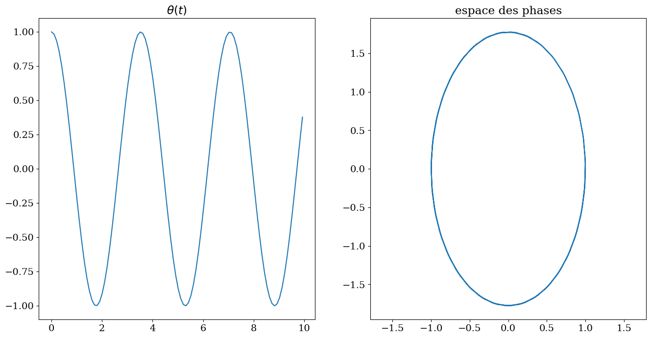
4.5. Probleme non raide#
Oscillateur harmonique : pendule simple $\( \frac{d^2\theta}{dt^2} + {\omega_0}^2 \theta = 0 \)$
# parametres
g = 10.
l = 1.
omega0=np.sqrt(g/l)
# rhs dY/dt = rhs(t,Y)
nit = 0
def rhs(t,y,dy):
    global omega0,nit
    nit  += 1
    dy[0] =  y[1]
    dy[1] = -omega0*y[0]
    return
# C.I.
y0 = np.array([1.0,0.0])
t0 = 0.0
tfinal = 10*np.pi/omega0
4.6. méthode RK avec ode#
SOLVER = 'dopri5'
t      = np.linspace(0, tfinal,100)
initial_values = y0
ode_solver = ode(SOLVER, rhs, old_api=False)
nit = 0
output = ode_solver.solve(t, initial_values)
print("Nbre d'appel a rhs: ",nit)
output.message
Nbre d'appel a rhs: 1324
'computation successful'
output
SolverReturn(flag=<StatusEnumDOP.SUCCESS: 1>, values=SolverVariables(t=array([0.        , 0.10034938, 0.20069875, 0.30104813, 0.40139751,
       0.50174688, 0.60209626, 0.70244563, 0.80279501, 0.90314439,
       1.00349376, 1.10384314, 1.20419252, 1.30454189, 1.40489127,
       1.50524065, 1.60559002, 1.7059394 , 1.80628878, 1.90663815,
       2.00698753, 2.1073369 , 2.20768628, 2.30803566, 2.40838503,
       2.50873441, 2.60908379, 2.70943316, 2.80978254, 2.91013192,
       3.01048129, 3.11083067, 3.21118005, 3.31152942, 3.4118788 ,
       3.51222817, 3.61257755, 3.71292693, 3.8132763 , 3.91362568,
       4.01397506, 4.11432443, 4.21467381, 4.31502319, 4.41537256,
       4.51572194, 4.61607132, 4.71642069, 4.81677007, 4.91711944,
       5.01746882, 5.1178182 , 5.21816757, 5.31851695, 5.41886633,
       5.5192157 , 5.61956508, 5.71991446, 5.82026383, 5.92061321,
       6.02096259, 6.12131196, 6.22166134, 6.32201071, 6.42236009,
       6.52270947, 6.62305884, 6.72340822, 6.8237576 , 6.92410697,
       7.02445635, 7.12480573, 7.2251551 , 7.32550448, 7.42585386,
       7.52620323, 7.62655261, 7.72690198, 7.82725136, 7.92760074,
       8.02795011, 8.12829949, 8.22864887, 8.32899824, 8.42934762,
       8.529697  , 8.63004637, 8.73039575, 8.83074513, 8.9310945 ,
       9.03144388, 9.13179325, 9.23214263, 9.33249201, 9.43284138,
       9.53319076, 9.63354014, 9.73388951, 9.83423889, 9.93458827]), y=array([[ 1.        ,  0.        ],
       [ 0.98412014, -0.31565107],
       [ 0.93698491, -0.62127716],
       [ 0.86009131, -0.90717166],
       [ 0.75588145, -1.16425465],
       [ 0.62766501, -1.38436124],
       [ 0.47951412, -1.56050091],
       [ 0.31613399, -1.68707952],
       [ 0.14271354, -1.76007697],
       [-0.03523945, -1.77717488],
       [-0.21207324, -1.73783023],
       [-0.38217165, -1.64329258],
       [-0.5401324 , -1.49656444],
       [-0.68093869, -1.30230583],
       [-0.80011857, -1.06668637],
       [-0.89388691, -0.79718925],
       [-0.95926565, -0.50237363],
       [-0.9941784 , -0.19160278],
       [-0.99751632,  0.12525333],
       [-0.96917342,  0.43813142],
       [-0.91004984,  0.73709459],
       [-0.82202334,  1.01264784],
       [-0.70788961,  1.25603968],
       [-0.57127351,  1.45954006],
       [-0.41651393,  1.61668587],
       [-0.24852599,  1.7224862 ],
       [-0.07264494,  1.77358086],
       [ 0.1055433 ,  1.7683471 ],
       [ 0.28037951,  1.70695114],
       [ 0.44631095,  1.5913429 ],
       [ 0.59806768,  1.42519407],
       [ 0.73082994,  1.21378148],
       [ 0.84038126,  0.96381955],
       [ 0.92324231,  0.68324698],
       [ 0.97678145,  0.38097468],
       [ 0.99929829,  0.06660275],
       [ 0.99007771, -0.24988448],
       [ 0.94941254, -0.55843544],
       [ 0.8785943 , -0.84925065],
       [ 0.77987215, -1.1130939 ],
       [ 0.65638149, -1.34158561],
       [ 0.51204434, -1.52746894],
       [ 0.35144481, -1.6648403 ],
       [ 0.1796835 , -1.7493368 ],
       [ 0.00221549, -1.77827487],
       [-0.17532288, -1.75073544],
       [-0.34729305, -1.66759316],
       [-0.50823329, -1.53148859],
       [-0.65303218, -1.34674438],
       [-0.77709096, -1.11922796],
       [-0.87646955, -0.85616518],
       [-0.94801172, -0.56591084],
       [-0.98944531, -0.25768334],
       [-0.9994544 ,  0.05872811],
       [-0.97772111,  0.37327437],
       [-0.92493567,  0.67596555],
       [-0.84277454,  0.95718824],
       [-0.73384713,  1.20801092],
       [-0.60161295,  1.42046751],
       [-0.45027171,  1.58781046],
       [-0.28462998,  1.704725  ],
       [-0.10994848,  1.76749797],
       [ 0.06822495,  1.77413571],
       [ 0.24423158,  1.72442741],
       [ 0.41248148,  1.61995178],
       [ 0.56763109,  1.46402695],
       [ 0.70475289,  1.26160505],
       [ 0.81949195,  1.01911493],
       [ 0.90820417,  0.74425801],
       [ 0.96807209,  0.44576368],
       [ 0.99719432,  0.13311202],
       [ 0.99464594, -0.18376724],
       [ 0.96050789, -0.4948101 ],
       [ 0.89586439, -0.79013793],
       [ 0.80276849, -1.06037121],
       [ 0.68417689, -1.2969274 ],
       [ 0.54385604, -1.49229355],
       [ 0.38626247, -1.64026488],
       [ 0.21640131, -1.73614187],
       [ 0.03966732, -1.77687949],
       [-0.1383265 , -1.76118393],
       [-0.31192711, -1.68955367],
       [-0.475621  , -1.56426367],
       [-0.6242093 , -1.3892931 ],
       [-0.7529729 , -1.17019898],
       [-0.85782229, -0.91393968],
       [-0.93542749, -0.62865392],
       [-0.98332378, -0.32340229],
       [-0.99998999, -0.00787951],
       [-0.9848968 ,  0.30789353],
       [-0.93852358,  0.61388796],
       [-0.86234311,  0.90038548],
       [-0.75877487,  1.15828702],
       [-0.63110817,  1.37940169],
       [-0.48339764,  1.55670695],
       [-0.32033455,  1.68457165],
       [-0.14709773,  1.75893483],
       [ 0.03081088,  1.77743475],
       [ 0.20774094,  1.73948386],
       [ 0.3780732 ,  1.64628745]])), errors=SolverVariables(t=None, y=None), roots=SolverVariables(t=None, y=None), tstop=SolverVariables(t=None, y=None), message='computation successful')
4.6.1. Tracer de la solution#
T=output.values.t[:]
Y=output.values.y[:,0]
dY=output.values.y[:,1]
plt.figure(figsize=(16,8))
plt.subplot(1,2,1)
plt.plot(T,Y)
plt.title("$\\theta(t)$")
plt.subplot(1,2,2)
plt.plot(Y,dY)
plt.axis('equal')
plt.title("espace des phases")
Text(0.5, 1.0, 'espace des phases')
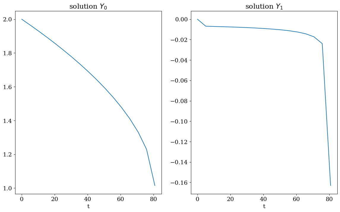
4.7. Problème raide: réaction chimique#
soit
plus \(\mu\) est grand, plus le système est difficile !
mu=None
def rhs(t,Y,dY):
    global mu,nit
    nit  += 1
    dY[0] = Y[1]
    dY[1] = mu*(1-Y[0]**2)*Y[1]-Y[0]
    return
# parametres
mu   = 10
# cas raide
mu   = 100.0
#mu   = 1000.0
tmax = 100.
# temps plus long
tmax = 500
t0 = 0.0
y0 = np.array([2. , 0.])
# définition du model et utilisation du solveur
SOLVER = 'dopri5'
t      = np.linspace(0, tmax,100)
initial_values = y0
#ode_solver = ode(SOLVER, rhs, old_api=False, max_steps=5000)
ode_solver = ode(SOLVER, rhs, old_api=False)
nit = 0
output = ode_solver.solve(t, initial_values)
print("Nbre d'appel a rhs: ",nit)
if output.errors.t:
    print ('Error: ', output.message, 'Error at time', output.errors.t)
output.message
Nbre d'appel a rhs:  30168
Error:  Unexpected idid, check warnings for info Error at time 85.85858585858585
/home/buffat/venvs/jupyter/lib/python3.10/site-packages/scipy/integrate/_ode.py:438: UserWarning: dopri5: larger nsteps is needed
  self._y, self.t = mth(self.f, self.jac or (lambda: None),
'Unexpected idid, check warnings for info'
T = output.values.t
Y = output.values.y
plt.figure(figsize=(14,8))
plt.subplot(1,2,1)
plt.plot(T,Y[:,0])
plt.title("solution $Y_0$")
plt.xlabel('t');
plt.subplot(1,2,2)
plt.plot(T,Y[:,1])
plt.title("solution $Y_1$")
plt.xlabel('t');
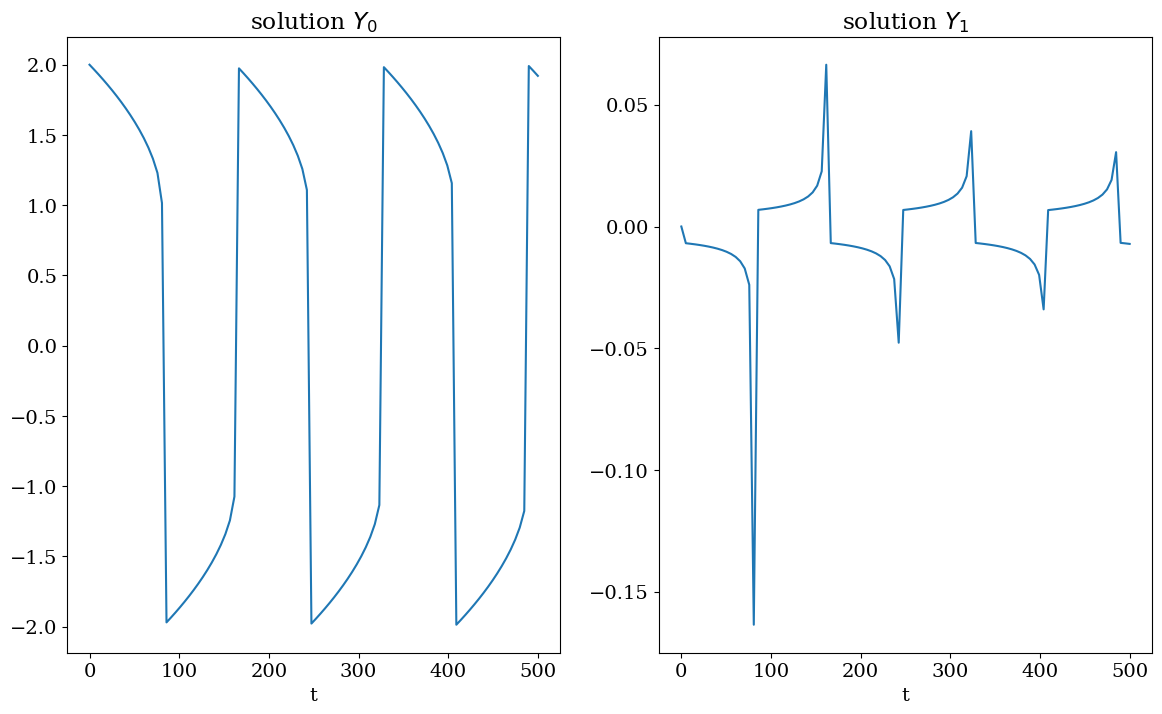
4.7.1. solveur raide#
# définition du model et utilisation du solveur
#tmax = 2000
SOLVER = 'cvode'
t      = np.linspace(0, tmax,100)
initial_values = y0
ode_solver = ode(SOLVER, rhs, old_api=False, max_steps=5000)
nit = 0
output = ode_solver.solve(t, initial_values)
print("Nbre d'appel a rhs: ",nit)
if output.errors.t:
    print ('Error: ', output.message, 'Error at time', output.errors.t)
output.message
Nbre d'appel a rhs: 5027
'Successful function return.'
T = output.values.t
Y = output.values.y
plt.figure(figsize=(14,8))
plt.subplot(1,2,1)
plt.plot(T,Y[:,0])
plt.title("solution $Y_0$")
plt.xlabel('t');
plt.subplot(1,2,2)
plt.plot(T,Y[:,1])
plt.title("solution $Y_1$")
plt.xlabel('t');
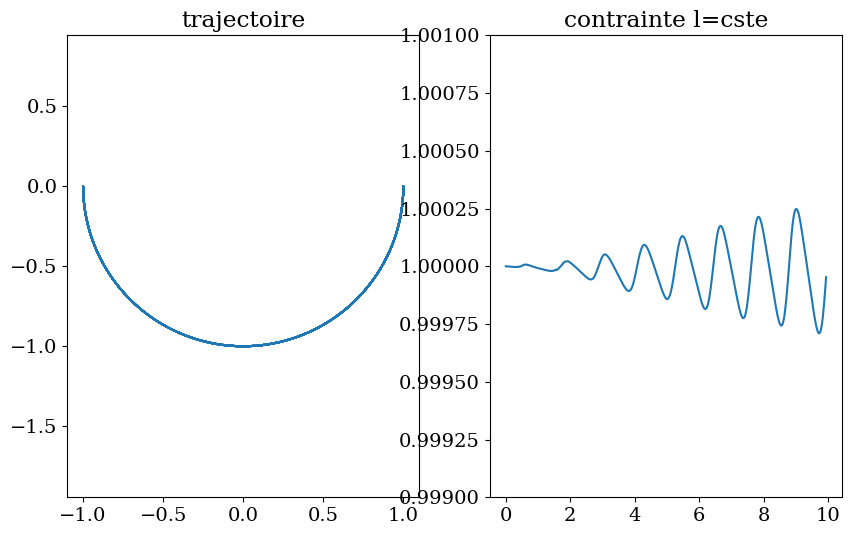
4.8. DAE#
pendule simple avec contrainte: \(x^2+y^2=l^2\)
Problème initiale: DAE d’ordre 2
Transformation en DAE d’ordre 1, mais d’index 2
# EDO sous forme implicite avec contrainte
# parametre de penalisation
beta=0.0
#beta=1.0e2
# Y = [x,y,dx,dy,lambda]
def residu(t,Y,dY,res):
    global nit
    nit += 1
    res[0]=dY[0]-Y[2]
    res[1]=dY[1]-Y[3]
    res[2]=dY[2]+2*Y[4]*Y[0]
    res[3]=dY[3]+2*Y[4]*Y[1]+g
    res[4]=Y[2]**2+Y[3]**2-2*Y[4]*l-g*Y[1] + beta*(Y[0]*Y[0]+Y[1]*Y[1]-l*l)
    return
# C.I.
t0 = 0.0
Y0 = [1.0, 0.0, 0.0, 0.0, 0.0]
dY0= [0.0, 0.0, 0.0, -g, 0.0]
# temps
periode=2*np.pi/np.sqrt(g/l)
tfinal = 5*periode
N=500
solver = dae('ida', residu, compute_initcond='yp0',
             first_step_size=1e-18,
             atol=1e-6,rtol=1e-6,
             algebraic_vars_idx=[4],
             old_api=False, max_steps=5000)
t = np.linspace(0,tfinal,N)
nit = 0
solution = solver.solve(t,Y0,dY0)
print("Nbre d'appel a rhs: ",nit)
if solution.errors.t:
    print ('Error: ', solution.message, 'Error at time', solution.errors.t)
solution.message
Nbre d'appel a rhs: 2491
'Successful function return.'
T = solution.values.t
Y = solution.values.y
plt.figure(figsize=(10,6))
plt.subplot(1,2,1)
plt.plot(Y[:,0],Y[:,1])
plt.axis('equal')
plt.title('trajectoire')
plt.subplot(1,2,2)
plt.plot(T,Y[:,0]**2+Y[:,1]**2)
eps=0.001
plt.ylim([l*(1.-eps),l*(1.+eps)])
plt.title('contrainte l=cste')
Text(0.5, 1.0, 'contrainte l=cste')
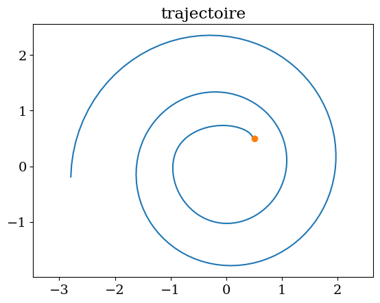
4.9. probleme bille#

  c = cos(omega*(t+t0))
  s = sin(omega*(t+t0))
fr coefficiant de frottement
equations
u1' =   u2
u2' = - fr*u2 + lambda*c
u3' =   u4
u4' = - fr*u4 - lambda*s + g
contrainte sur la bille B : OB=(u1,u3) // tige (c,s)
0 = c*u3 - s*u1
def rhs(t,u):
    s = np.sin(t+np.pi/4)
    c = np.cos(t+np.pi/4)
    up = np.zeros(5)
    up[0] =   u[1]
    up[1] = - 10*u[1] + u[4]*s
    up[2] =   u[3]
    up[3] = - 10*u[3] - u[4]*c + 1
    # contrainte
    g     =  c*u[2] - s*u[0]
    gp    =  c*(u[3] - u[0]) + s*( - u[1] - u[2])
    gpp   =  c*(up[3] - up[0] - u[1] - u[2]) \
           + s*(- up[1] - up[2] - u[3] + u[0])
    # penalisation
    up[4] = gpp + 20*gp + 100*g
    return up
# residu
def residu(t,u,du,res):
    global nit
    nit+=1
    res[:] = du - rhs(t,u)
    return
# cdt initiale
t0 = 0.0
Y0 = np.array([0.5,-0.5,0.5,0.5,0]);
dY0 = rhs(t0,Y0)
tfinal=15
N = 200
solver = dae('ida', residu, compute_initcond='yp0',
             first_step_size=1e-18,
             atol=1e-6,rtol=1e-6,
             algebraic_vars_idx=[4],
             old_api=False, max_steps=5000)
t = np.linspace(0,tfinal,N)
nit = 0
solution = solver.solve(t,Y0,dY0)
print("Nbre d'appel a rhs: ",nit)
if solution.errors.t:
    print ('Error: ', solution.message, 'Error at time', solution.errors.t)
solution.message
Nbre d'appel a rhs: 766
'Successful function return.'
T = solution.values.t
Y = solution.values.y
plt.plot(Y[:,0],Y[:,2])
plt.plot(Y0[0],Y0[2],'o')
plt.title("trajectoire")
plt.axis('equal');
#
# animation
# =========
fig=plt.figure()
ax = fig.add_subplot(111, aspect='equal')
ax.set_axis_off()
ax.set_xlim((-3.,3.))
ax.set_ylim((-3.,3.))
plt.title('bille')
fig.set_facecolor("#ffffff")
line1, = ax.plot([], [], '-k', lw=2)
line, = ax.plot([], [], 'o', lw=1 , markersize=30)
def init():
    line.set_data([], [])
    line1.set_data([], [])
    return line,
def animate(i):
    x = Y[i,0]
    y = Y[i,2]
    thisx = [x]
    thisy = [y]
    line1.set_data([0.,3*np.cos((T[i]+np.pi/4))],[0.,3*np.sin((T[i]+np.pi/4))])
    line.set_data(thisx, thisy)
    return line,

anim = animation.FuncAnimation(fig, animate, np.arange(1, N), interval=50, blit=True, init_func=init);

HTML(anim.to_html5_video())