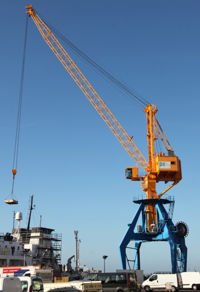
Planification: mouvement d’une grue

Contenu

5. Planification: mouvement d’une grue#

Marc BUFFAT, département mécanique, UCB Lyon 1

grue

%matplotlib inline
import numpy as np
import sympy as sp
import matplotlib.pyplot as plt
plt.rc('font', family='serif', size='14')
from IPython.display import display, Markdown, clear_output
def printmd(string):
    display(Markdown(string))
from metakernel import register_ipython_magics
register_ipython_magics()
from sympy.physics.vector import init_vprinting
init_vprinting()

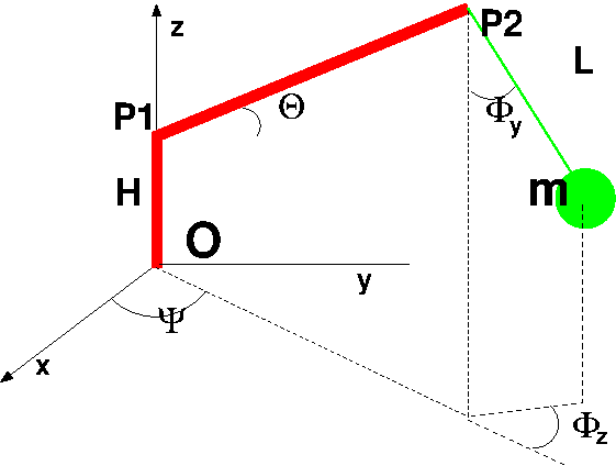
5.1. Description#

repere fixe en O, $R_O$
Bras $P_1P_2$ fixe en P1 (a H de O suivant Z) cylindre de longueur Lb, de masse Mb et de rayon a
repere $R_b$ lié au bras (// a $R_b.x$)
rotation $\psi(t)$ autour de $R_O.z$
rotation de $\theta(t)$ autour de $R_a.y$ (attention angle <0)
masse m accroché à $P_2$ (extrémité du bras) par un cable de longueur L (2 rotations $\phi_y$,$\phi_z$)

schema

5.2. Parametres et repéres#

# parametres
from sympy.physics.mechanics import dynamicsymbols, Point, ReferenceFrame
from sympy.physics.mechanics import Particle, RigidBody, Lagrangian, LagrangesMethod
theta, psi, phiy, phiz     = dynamicsymbols('theta psi phi_y phi_z')
thetap, psip, phiyp, phizp = dynamicsymbols('theta psi phi_y phi_z',level=1)
H, Lb, Mb, alpha, omega    = sp.symbols('H L_b M_b alpha omega')
# rayon barre 1/10 Lb
a = Lb/10
# masse m de la masse
m = 10*Mb
# longueur du cable
l = alpha*Lb
# force de gravite 
g = omega**2*l

# repêres barre
O = Point('O')
RO = ReferenceFrame('R_O')
P1 = Point('P1')
P1.set_pos(O,H*RO.z)
R1 = ReferenceFrame('R_1')
R1.orient(RO,'Axis',[psi, RO.z])
Rb = ReferenceFrame('R_b')
Rb.orient(R1,'Axis',[theta, R1.y])
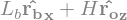
P2 = Point('P2')
P2.set_pos(P1,Lb*Rb.x)
display("OP2=",P2.pos_from(O))
G = Point('G')
G.set_pos(P1,Lb/2*Rb.x)
display("OG=",G.pos_from(O))

'OP2='

../../_images/551df26311fdbff19938c3b28cc65a6f13864e05b7ca170a3bdc052ec6cb00a6.png

'OG='

../../_images/45e689ce0fafc9e8b48060ab067a453b230c0451793bb736d9652c0bc113476d.png

# repere masse (rotation phi)
R2 = ReferenceFrame('R_2')
R2.orient(R1,'Axis',[phiz, R1.z])
Rm  = ReferenceFrame('R_m')
Rm.orient(R2,'Axis',[phiy, R2.y])
M = Point('M')
M.set_pos(P2,-l*Rm.z)
display("OM=",M.pos_from(O))

'OM='

../../_images/9f1943eeab374187fc900573eb076833565171de7d9a4bc577c98334067bac25.png

5.3. Cinématique#

# calcul directe
from sympy.physics.vector import express,time_derivative
display("OM=",express(M.pos_from(O),RO))
display("VM=",express(time_derivative(M.pos_from(O),RO),RO).simplify())

'OM='

../../_images/5242068052d22ce0c9e31ec45e965635d4b59a8fce9a28fb69518be414cc6035.png

'VM='

../../_images/94efd2ebc54759d008f2e6bde4eab476b5b9e549d4974bfbb8948ec6d4c3ded2.png

# inertie
from sympy.physics.mechanics import inertia
Ix = Mb*a**2/2
Iy = Mb*a**2/4 + Mb*Lb**2/12
IG = inertia(Rb,Ix,Iy,Iy)
display("IG=",IG)

'IG='

../../_images/b65840db8439d62cc0401e65810c686a4721ed6fd542d0b49071b400c4edd4f7.png

# vitesse
O.set_vel(RO,0.)
P1.set_vel(RO,0.)
P2.set_vel(Rb,0.)
G.set_vel(Rb,0.)
# composition des vitesses
P2.v2pt_theory(P1,RO,Rb)
G.v2pt_theory(P1,RO,Rb)
display("VP2=",P2.vel(RO),"VG=",G.vel(RO))
display("dans Rb=",P2.vel(Rb),G.vel(Rb))

'VP2='

../../_images/4c1b6496d79913a7e132134a914d47bb83561665c39fbd9a94b9fc6003d8c435.png

'VG='

../../_images/4bd9025f1ad97d406289ea5fbcdc94be4bf0d3a43692ade826f6021fca144eb7.png

'dans Rb='

../../_images/702ba12f4bf2cef7092842f0bdd4dc2b8bfdc07d13bc79cc481075cd1cc7c88c.png

# vitesse de M
M.set_vel(Rm,0.)
M.v2pt_theory(P2,RO,Rm)
display("VM=",M.vel(RO))

'VM='

../../_images/c4b0e7d1c1ac202bb964e5361b40e4ef5d4cf96a0a735acf7e37e61eb060260a.png

5.4. Formalisme de Lagrange#

systeme = Barre + Masse

Masse = Particle('Masse',M,m)
Barre = RigidBody('Barre',G,Rb,Mb,(IG,G))

display("Ec Barre=",Barre.kinetic_energy(RO).simplify())
display("Ec Masse=",Masse.kinetic_energy(RO).simplify())

'Ec Barre='

../../_images/8c4965e9685ee774339ca6d98b1080a3613145685e972f098f019ffcc2abc2d9.png

'Ec Masse='

../../_images/8ada9cc7d0760d8b0591d1ffc5fdc06f895605e9d62a80e3cfab62f6ede11133.png

# reference en P1
Barre.potential_energy = Mb*g*G.pos_from(P1).dot(RO.z)
display("Ep Barre:",Barre.potential_energy)
Masse.potential_energy = m*g*M.pos_from(P1).dot(RO.z)
display("Ep Masse:",Masse.potential_energy)

'Ep Barre:'

../../_images/d151df431147cbf0d84815954ec35211835ae6c4d0fc7403251c512f5b2f0da1.png

'Ep Masse:'

../../_images/fa97592a84a14b8629489dd6d1bccc73ef02a84d404a18da5e3cea0f601533d8.png

# calcul lagrangien
La = Lagrangian(RO,Barre,Masse)
La = La/(Lb**2*Mb)
La = La.simplify()
display("La=",La)

'La='

../../_images/6f1eb9d18bf2d0843acbb512f92b5ca6cb9cce3a61afcd4e6a45eb960e0256fe.png

5.5. Cas $\theta=cste$ $\psi=cste$ (grue immobile)#

mouvement pendule 3D
oscillation pendule simple : $$\omega^2 = \frac{g}{l} $$
notebook Pendule3D

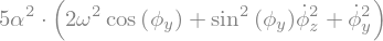
LLa = La.subs({theta:0,thetap:0,psi:0,psip:0})/(10*alpha**2)
LLa = LLa.simplify()
display("La=",LLa)

'La='

../../_images/0db20253da15d006d53fc61edb5b91c0246b64f99edd50deb5dda87c4e01b6cf.png

# equation lagrange
LLM = LagrangesMethod(LLa,[phiy,phiz],frame=RO)
Eq = LLM.form_lagranges_equations()
display(Eq)

../../_images/4947e0c44e30dc67eafe695868e4468ad215380e6d450c05b86b95aeb4e845be.png

# parametres
LL    = 2.0
Alpha = 1.0
Omega = np.sqrt(10./(Alpha*LL))
Tp    = 2*np.pi/Omega
print("T=",Tp,"Omega=",Omega)

T= 2.8099258924162904 Omega= 2.23606797749979

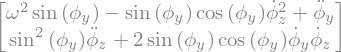
5.6. Cas $\theta=cste$ $\dot{\psi}=cste$#

cas grue en rotation

$\theta = \pi/4$
$\psi = kp\,t $

kp, t = sp.symbols('k_p t')
LLa = La.subs({theta:sp.pi/4,thetap:0,psi:kp*t,psip:kp})/(10)
LLa = LLa.simplify()
display("La=",LLa)

'La='

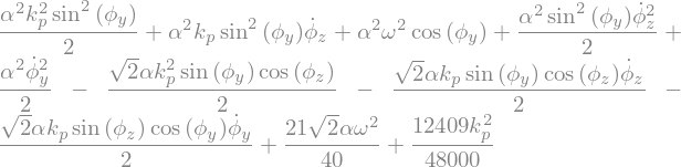
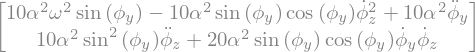
../../_images/ceb512312cf07a6c712d83c584f85fce513d30f4a56b2b3bbb800572ee6429f7.png

# equation lagrange
LLM = LagrangesMethod(LLa,[phiy,phiz],frame=RO)
Eq = LLM.form_lagranges_equations()
display("Lagrange:",Eq)

'Lagrange:'

../../_images/4a5f04a7fa3ffd7ad7a9615a06806c54f0f1324ef3a3fa40671085dfd173d1e3.png

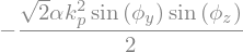
5.6.1. solution particulière#

La solution $\phi_y=cste$ et $\phi_z=cste$ conduit forcement a $\phi_z=0$

$\leadsto$ alignement de la masse avec la barre (dans le meme plan)

# solution Phiy=cste Phiz=cste
eq0=Eq[0].subs({phiy.diff(t,t):0}).subs({phiyp:0,phizp:0}).simplify()/alpha
eq1=Eq[1].subs({phiz.diff(t,t):0}).subs({phiyp:0,phizp:0}).simplify()
display(eq0,eq1)

../../_images/8c00840eb78d796685f247e9567279bd66e38e0499844cfe7747808f5e722ef8.png

../../_images/e2d90136061757840f9354ad47f6852696d0afd1e1a5543db0f5279e66622103.png

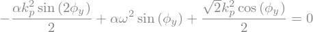
eq0=eq0.subs({phiz:0})
display(sp.Eq(eq0,0))

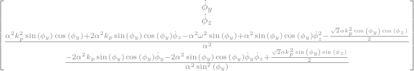
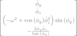
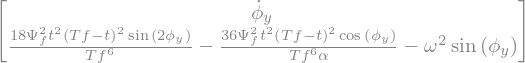
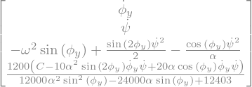
../../_images/b523c428fa01969502fe3b6a8178f76dbdf705b6ddcd7cbb0b7e7290570fa7e8.png

5.6.2. solution numérique#

transformation du système de Lagrange $$ A \dot{Y} = B $$ en $$ \dot{Y} = F(Y) $$

# resolution numérique
A=LLM.mass_matrix_full
B=LLM.forcing_full
FY = A.inv()*B
display("FY=",FY)

'FY='

../../_images/d8654c0fe087e86cf588f25e363e00b8ca8cd256d954dd795d49f94d3d60e8a1.png

# conversion en fonction python BY
smBY = sp.lambdify((phiy,phiz,phiyp,phizp,omega,alpha,kp),FY,'numpy')

# fonction F(Y)
def F(Y,t):
    '''second membre de l EDO dY/dt = F(Y) avec Y=[phiy,phiz,phiyp,phizp]'''
    global Omega,Alpha,Kp
    FF =smBY(Y[0],Y[1],Y[2],Y[3],Omega,Alpha,Kp)
    return FF[:,0]

# parametres
HH    = 1.0
LL    = 2.0
Alpha = 1.0
Omega = np.sqrt(10./(Alpha*LL))
Kp    = 1.
Tp    = 2*np.pi/Omega
print("T=",Tp,"Omega=",Omega)

T= 2.8099258924162904 Omega= 2.23606797749979

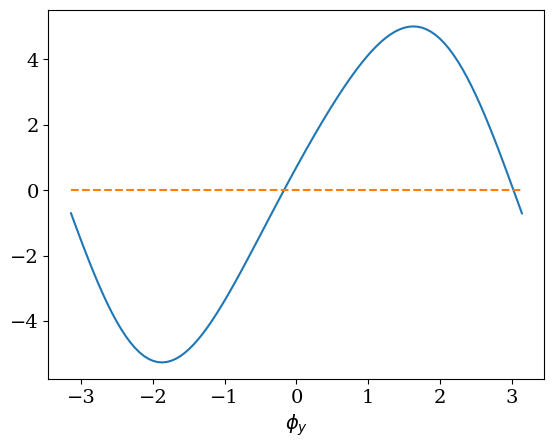
5.6.3. calcul solution particuliere phi=cste#

détermination de phiy pour phiz=0
2 racines proches de 0 et pi

# condition correspondant à l'équilibre phi=cste
Eq0=eq0.subs({alpha:Alpha,omega:Omega,kp:Kp})
display(Eq0)
EQ0=sp.lambdify(phiy,Eq0)

../../_images/b6d11fc1d1883b4f60c8353f1f5a953cbe2eae881c7fe4c14725a6932bfb2683.png

PHIY=np.linspace(-np.pi,np.pi,100)
YY = EQ0(PHIY)
plt.plot(PHIY,YY,label="eq0")
plt.plot(PHIY,np.zeros(PHIY.size),'--')
plt.xlabel("$\phi_y$");

../../_images/2b0fa06d5ce097f1b8fe1e98dd02ad7a4ffb410d68fb415fee876454cee51680.png

from scipy.optimize import fsolve
Phiy0=fsolve(EQ0,0.)[0]
Phiy1=fsolve(EQ0,np.pi)[0]
print("Racines Phiy0={:.3f} Phiy1={:.3f}".format(Phiy0,Phiy1))

Racines Phiy0=-0.174 Phiy1=3.024

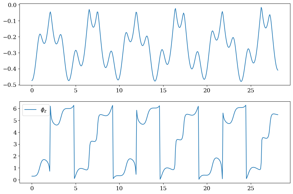
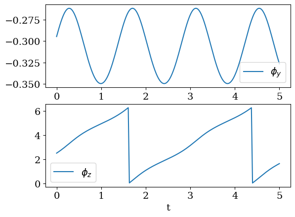
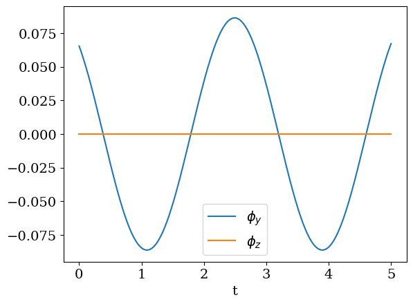
5.6.4. résolution numérique#

from scipy.integrate import odeint
# solution equilibre
Y0 = np.array([Phiy0,0.0,0.0,0.0])
# solution avec perturbation
Y0 = np.array([Phiy0-0.3,0.3,0.0,0.0])
print("F(Y0)=",F(Y0,0.))
T  = 10*Tp
N  = 400
tt = np.linspace(0,T,N)
sol = odeint(F,Y0,tt,atol=1.e-12,rtol=1.e-12)
PHIY = sol[:,0]
PHIZ = np.mod(sol[:,1],2*np.pi)

F(Y0)= [ 0.          0.          1.27641501 -0.45751735]

plt.figure(figsize=(12,8))
plt.subplot(2,1,1)
plt.plot(tt,PHIY,label='$\\phi_y$')
plt.subplot(2,1,2)
plt.plot(tt,PHIZ,label='$\\phi_z$')
plt.legend()

<matplotlib.legend.Legend at 0x7f7f2d114820>

../../_images/3c5e468c9b2f8a6e075f85972d926a1305c9db775c5570109ecec628f1a03484.png

# position de P2
P2x = sp.lambdify((theta,psi,Lb),express(P2.pos_from(O),RO).dot(RO.x),'numpy')
P2y = sp.lambdify((theta,psi,Lb),express(P2.pos_from(O),RO).dot(RO.y),'numpy')
P2z = sp.lambdify((theta,psi,Lb,H),express(P2.pos_from(O),RO).dot(RO.z),'numpy')
P2X = P2x(0.,Kp*tt,LL)
P2Y = P2y(0.,Kp*tt,LL)
P2Z = P2z(0.,Kp*tt,LL,HH)*np.ones(tt.size)

# et position de M
Mx = sp.lambdify((theta,psi,phiy,phiz,Lb,alpha),express(M.pos_from(O),RO).dot(RO.x),'numpy')
My = sp.lambdify((theta,psi,phiy,phiz,Lb,alpha),express(M.pos_from(O),RO).dot(RO.y),'numpy')
Mz = sp.lambdify((theta,psi,phiy,phiz,Lb,H,alpha),express(M.pos_from(O),RO).dot(RO.z),'numpy')
MX = Mx(0.,Kp*tt,PHIY,PHIZ,LL,Alpha)
MY = My(0.,Kp*tt,PHIY,PHIZ,LL,Alpha)
MZ = Mz(0.,Kp*tt,PHIY,PHIZ,LL,HH,Alpha)

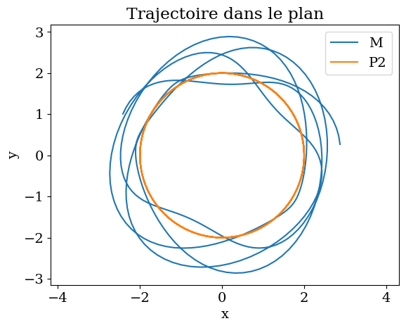
plt.title("Trajectoire dans le plan")
plt.plot(MX,MY,label="M")
plt.plot(P2X,P2Y,label="P2")
plt.xlabel('x')
plt.ylabel('y')
plt.legend()
plt.axis('equal');

../../_images/9ef5e65bcd19ec0b73f22b9277017fc9ac6e17b7319d56085d8076e0c89c54d3.png

# trajectoire en 3D
from validation.Pendule3D import TrajectoireBras3D

TrajectoireBras3D(P2X,P2Y,P2Z,MX,MY,MZ,HH,LL*1.5)

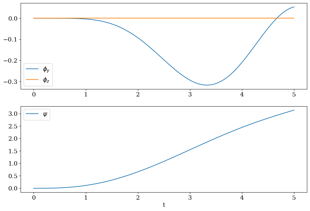
5.7. Etude d’un mouvement imposé#

etude du mouvement pour déplacer une charge d’un point A à B
cas $\theta=0$ et $\psi(t)$ imposée (interpolation degré 3 )

5.7.1. calcul de la loi horaire#

définition d’une loi horaire $\psi(t)$
polynôme $p(t)=a_0 + a_1 t + a_2 t^2 + a_3 t^3$
durée du mouvement $T$
conditions $p(0)=0, \dot{p}(0) = 0 , p(T)=\psi_f, \dot{p}(T)=0$

\[\psi(t) = \psi_f \frac{t^2 (3T-2t)}{T^3}\]

Psif , Tf  = sp.symbols('Psi_f Tf')
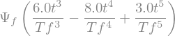
Psi = Psif*t**2*(3*Tf-2*t)/Tf**3
display("Psi=",Psi)
LLa = La.subs({theta:0,thetap:0, psi: Psi, psip : Psi.diff(t) })
display("La=",LLa.simplify())

'Psi='

../../_images/5f696f129777bb4cc9504e31dc0a25b31721d7670032254c8422b6a9fa3b7478.png

'La='

../../_images/497a854c71aa37bbafc556dca5d785190f92490bdb45db96ffba0bc839e569f8.png

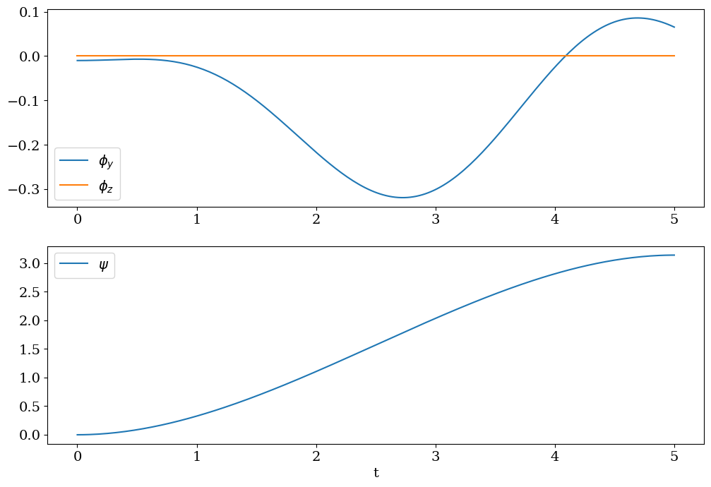
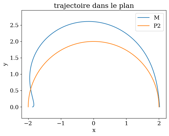
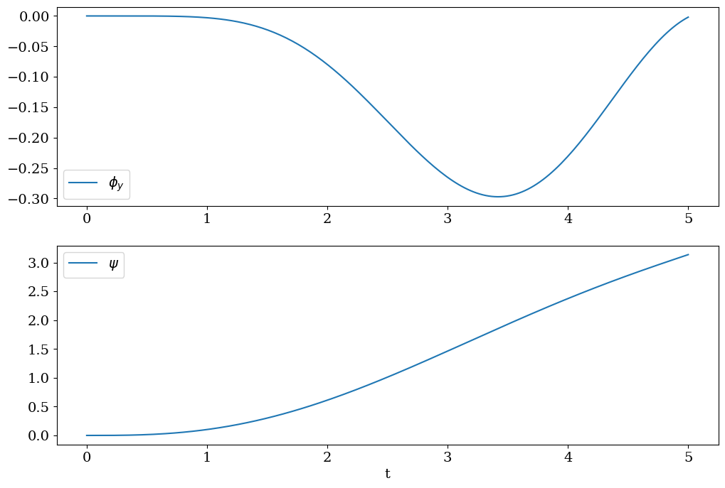
5.7.2. 1ere phase: mouvement de A a B#

LLM = LagrangesMethod(LLa,[phiy,phiz])
Eq = LLM.form_lagranges_equations()
display("Lagrange:",Eq)

'Lagrange:'

../../_images/9190a225499a1f7df4378b5493f3a5bb6342fc1931db2a25a941f3b620fbdf36.png

# conversion en EDO dY/dt = F(Y)
A=LLM.mass_matrix_full
B=LLM.forcing_full
FY=A.inv()*B
FY[2]=FY[2].simplify()
FY[3]=FY[3].simplify()
display("F(Y)=",FY)

'F(Y)='

../../_images/e041f7e16f38c54a8603efc4501a0b7521303a7b895cd69183df6387f51ab9be.png

# fonction BY
smBY = sp.lambdify((phiy,phiz,phiyp,phizp,t,alpha,omega,Psif,Tf),FY,'numpy')

# fonction F(Y)
def F(Y,t):
    '''second membre EDO dY/dt = F(Y) avec Y=[phiy,phiz,phiyp,phizp]'''
    global Alpha,Omega,PsiF,T
    FF =smBY(Y[0],Y[1],Y[2],Y[3],t,Alpha,Omega,PsiF,T)
    return FF[:,0]

# parametres
HH    = 1.0
LL    = 2.0
Alpha = 1.0
Omega = np.sqrt(10./(Alpha*LL))
Tp    = 2*np.pi/Omega
print("T=",Tp,"Omega=",Omega)
PsiF  = np.pi
# parcours lent
T = 20.
# parcours rapide
T = 5.
# parcours tres lent
#T = 80.

T= 2.8099258924162904 Omega= 2.23606797749979

# solution numerique
Y0 = np.array([-0.01,0.,0.,0.])
print(F(Y0,0.))
N  = 200
tt = np.linspace(0,T,N)
sol = odeint(F,Y0,tt)
PHIY = sol[:,0]
PHIZ = np.mod(sol[:,1],2*np.pi)
PSi  = sp.lambdify(t,Psi.subs({Tf:T,Psif:PsiF}),'numpy')
PSI  = PSi(tt)

[ 0.00000000e+00  0.00000000e+00  4.99991667e-02 -7.61534626e+01]

plt.figure(figsize=(12,8))
plt.subplot(2,1,1)
plt.plot(tt,PHIY,label='$\\phi_y$')
plt.plot(tt,PHIZ,label='$\\phi_z$')
plt.legend()
plt.subplot(2,1,2)
plt.plot(tt,PSI,label="$\psi$")
plt.xlabel('t')
plt.legend();

../../_images/c80484d224f35a26dbf2126ac3414b3885bc3be4ade4dc0b52c9cd7b2a1e0f92.png

# position de P2
P2X = P2x(0.,PSI,LL)
P2Y = P2y(0.,PSI,LL)
P2Z = P2z(0.,PSI,LL,HH)*np.ones(PSI.size)
# et de M
MX = Mx(0.,PSI,PHIY,PHIZ,LL,Alpha)
MY = My(0.,PSI,PHIY,PHIZ,LL,Alpha)
MZ = Mz(0.,PSI,PHIY,PHIZ,LL,HH,Alpha)

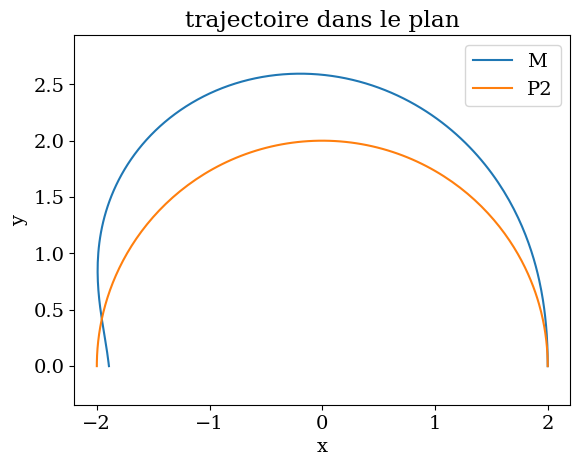
plt.title("trajectoire dans le plan")
plt.plot(MX,MY,label="M")
plt.plot(P2X,P2Y,label="P2")
plt.xlabel('x')
plt.ylabel('y')
plt.legend()
plt.axis('equal');

../../_images/b48889f5500416094101c775a532e9eefeb7f19827e3436d754014835f13be5b.png

# trajectoire 3D
TrajectoireBras3D(P2X,P2Y,P2Z,MX,MY,MZ,HH,LL*1.5)

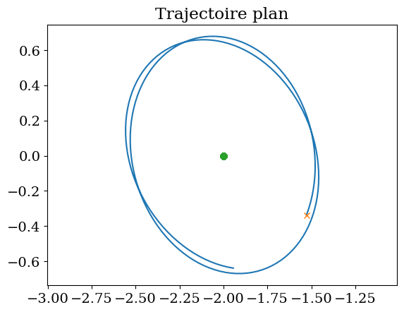
5.7.3. 2ieme phase: mouvement à la position finale#

# solution apres arret (pendule)
LLa = La.subs({theta:0,thetap:0, psi: Psif, psip : 0 })
display("La=",LLa.simplify())

'La='

../../_images/6fe75cd79b8186b5be12b388a9f92a875186144061565be99961cb50e64c3e80.png

LLM = LagrangesMethod(LLa,[phiy,phiz])
Eq = LLM.form_lagranges_equations()
display(Eq)

../../_images/989d2a6bcc1bdb91bb1e0f4beae6bb96fc2be3293f63e985305e5a7778a276bb.png

# transformation EDO dY/dt = F(Y)
A=LLM.mass_matrix_full
B=LLM.forcing_full
FY = A.inv()*B
FY[2]=FY[2].simplify()
FY[3]=FY[3].simplify()
display("FY=",FY)

'FY='

../../_images/0dbb83ec2d3a70c02be5f125d46e2f25a08a73b4951c57dde6c8798564fa22b3.png

# fonction BY
smBYf = sp.lambdify((phiy,phiz,phiyp,phizp,omega),FY,'numpy')

# fonction Ff(Y)
def Ff(Y,t):
    '''2nd membre de l EDO  dY/dt = F(Y)'''
    global Omega
    FF =smBYf(Y[0],Y[1],Y[2],Y[3],Omega)
    return FF[:,0]

# resolution numérique
Y0f = sol[-1,:]
print(Ff(Y0,0.))
ttf  = np.linspace(T,2*T,N)
solf = odeint(Ff,Y0f,ttf)
PHIY = solf[:,0]
PHIZ = np.mod(solf[:,1],2*np.pi)

[0.         0.         0.04999917 0.        ]

plt.subplot(2,1,1)
plt.plot(tt,PHIY,label='$\\phi_y$')
plt.legend()
plt.subplot(2,1,2)
plt.plot(tt,PHIZ,label='$\\phi_z$')
plt.legend()
plt.xlabel('t');

../../_images/a129929bbb7a1c6477dda948288f00f19093c2b299358c7b2936bdd4933fb520.png

# position de P2 et M
P2X = P2x(0.,PsiF,LL)*np.ones(PHIY.size)
P2Y = P2y(0.,PsiF,LL)*np.ones(PHIY.size)
P2Z = P2z(0.,PsiF,LL,HH)*np.ones(PHIY.size)
MX = Mx(0.,PsiF,PHIY,PHIZ,LL,Alpha)
MY = My(0.,PsiF,PHIY,PHIZ,LL,Alpha)
MZ = Mz(0.,PsiF,PHIY,PHIZ,LL,HH,Alpha)

plt.plot(MX,MY)
plt.plot(MX[0],MY[0],'x')
plt.plot(P2X,P2Y,'o')
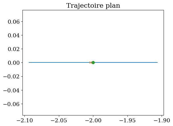
plt.title("Trajectoire plan")
plt.axis('equal');

../../_images/ae7bd78c532ab9d75519a50044a0760c72173b969eaa3be52f48213afd5b8456.png

# trajectoire 3D
TrajectoireBras3D(P2X,P2Y,P2Z,MX,MY,MZ,HH,LL*1.5)

5.8. Utilisation d’un cable anti-rotation#

un câble anti-giratoire empêche la rotation autour de z. Par un système d’assemblage de torons enroullés dans des sens opposé, le cable résistera à la rotation et ainsi la charge soulevée ne tournera pas sur elle-même. Ce type de câble est systèmatiquement utilisé dans les grues à tour ou grues de chantier. $$\dot{\phi_z} = 0$$

LLa = (La.subs({theta:0,thetap:0, psi: Psi, psip : Psi.diff(t), phiz:0, phizp:0 })).simplify()
display("La=",LLa)

'La='

../../_images/478bd19512e7e8d820bb46919b79ef1e3ab75c582c58c881d61d7531033d26b4.png

5.8.1. premiere phase A vers B#

LLM = LagrangesMethod(LLa,[phiy])
Eq = LLM.form_lagranges_equations()
display(Eq)

../../_images/680cd4ce64ab23a98f3f4b522195ded8c5a4c5069e887f4b38d1bd2794e73930.png

# transformation EDO dY/dt = F(Y)
A=LLM.mass_matrix_full
B=LLM.forcing_full
FY = A.inv()*B
FY[1] = FY[1].simplify()
display("FY=",FY)

'FY='

../../_images/3d40a075ad49c869a919175b9fafb6e6b92417289b9a9c749d860a58b6f89efb.png

# fonction BY
smBY = sp.lambdify((phiy,phiyp,t,alpha,omega,Psif,Tf),FY,'numpy')

# fonction F(Y)
def F(Y,t):
    '''second membre EDO dY/dt = F(Y) avec Y=[phiy,phiyp]'''
    global Alpha,Omega,PsiF,T
    FF =smBY(Y[0],Y[1],t,Alpha,Omega,PsiF,T)
    return FF[:,0]

# solution numerique
print("parametres:",Alpha,Omega,PsiF,T)
Y0 = np.array([-0.01,0.])
print(F(Y0,0.))
N  = 200
tt = np.linspace(0,T,N)
sol = odeint(F,Y0,tt)
PHIY = sol[:,0]
PHIZ = np.zeros(tt.size)
PSi  = sp.lambdify(t,Psi.subs({Tf:T,Psif:PsiF}),'numpy')
PSI  = PSi(tt)

parametres: 1.0 2.23606797749979 3.141592653589793 5.0
[0.         0.04999917]

plt.figure(figsize=(12,8))
plt.subplot(2,1,1)
plt.plot(tt,PHIY,label='$\\phi_y$')
plt.plot(tt,PHIZ,label='$\\phi_z$')
plt.legend()
plt.subplot(2,1,2)
plt.plot(tt,PSI,label="$\psi$")
plt.xlabel('t')
plt.legend();

../../_images/ee8e30480852e5d8d9af113e2f540a963794b73d1b0fbe01b02aaa788cc6885d.png

# position de P2
P2X = P2x(0.,PSI,LL)
P2Y = P2y(0.,PSI,LL)
P2Z = P2z(0.,PSI,LL,HH)*np.ones(PSI.size)
# et de M
MX = Mx(0.,PSI,PHIY,PHIZ,LL,Alpha)
MY = My(0.,PSI,PHIY,PHIZ,LL,Alpha)
MZ = Mz(0.,PSI,PHIY,PHIZ,LL,HH,Alpha)

plt.title("trajectoire dans le plan")
plt.plot(MX,MY,label="M")
plt.plot(P2X,P2Y,label="P2")
plt.xlabel('x')
plt.ylabel('y')
plt.legend()
plt.axis('equal');

../../_images/3e675482cc1c40396e8eeed77f4fdbd53225546ddc2cd39d2a3acb9102cf0799.png

# trajectoire 3D
TrajectoireBras3D(P2X,P2Y,P2Z,MX,MY,MZ,HH,LL*1.5)

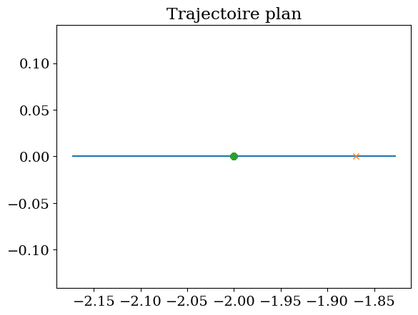
5.8.2. seconde phase#

# solution apres arret (pendule)
LLa = La.subs({theta:0,thetap:0, psi: Psif, psip : 0, phiz:0, phizp:0})
display("La=",LLa.simplify())

'La='

../../_images/1d485e7d2ade9635b4174ef17e827887d77c3cddf6243c2a68eb0cc17cc7f8ba.png

LLM = LagrangesMethod(LLa,[phiy])
Eq = LLM.form_lagranges_equations()
display(Eq)

../../_images/a8098eda325ae9bbbacea3b12e4018779654450ea13f7e6c9a7356d1f048594d.png

# transformation EDO dY/dt = F(Y)
A=LLM.mass_matrix_full
B=LLM.forcing_full
FY = A.inv()*B
FY[1]=FY[1].simplify()
display("FY=",FY)

'FY='

../../_images/34ba469617759d10f079bb0a1e456dc70f64a866e6c048685ad9fd9137fad904.png

# fonction BY
smBYf = sp.lambdify((phiy,phiyp,omega),FY,'numpy')

# fonction Ff(Y)
def Ff(Y,t):
    '''2nd membre de l EDO  dY/dt = F(Y)'''
    global Omega
    FF =smBYf(Y[0],Y[1],Omega)
    return FF[:,0]

# resolution numérique
Y0f = sol[-1,:]
print(Ff(Y0,0.))
ttf  = np.linspace(T,2*T,N)
solf = odeint(Ff,Y0f,ttf)
PHIY = solf[:,0]
PHIZ = np.zeros(ttf.size)

[0.         0.04999917]

plt.plot(tt,PHIY,label='$\\phi_y$')
plt.plot(tt,PHIZ,label='$\\phi_z$')
plt.legend()
plt.xlabel('t');

../../_images/13d601c81722ba7ab2a7fb6b1b850a48e4aa669fd40e28e73f1f21cba895cde4.png

# position de P2 et M
P2X = P2x(0.,PsiF,LL)*np.ones(PHIY.size)
P2Y = P2y(0.,PsiF,LL)*np.ones(PHIY.size)
P2Z = P2z(0.,PsiF,LL,HH)*np.ones(PHIY.size)
MX = Mx(0.,PsiF,PHIY,PHIZ,LL,Alpha)
MY = My(0.,PsiF,PHIY,PHIZ,LL,Alpha)
MZ = Mz(0.,PsiF,PHIY,PHIZ,LL,HH,Alpha)

plt.plot(MX,MY)
plt.plot(MX[0],MY[0],'x')
plt.plot(P2X,P2Y,'o')
plt.title("Trajectoire plan")
plt.axis('equal');

../../_images/1ac8367bab8627c77fbb1e7a9498f6ed18f881e39e400cd305af1cde94924062.png

# trajectoire 3D
TrajectoireBras3D(P2X,P2Y,P2Z,MX,MY,MZ,HH,LL*1.5)

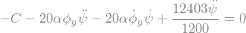
5.9. Contrôle avec cable anti-rotation#

On veut finaliser le contrôle du mouvement en contrôlant le couple $C$ qui impose la rotation du bras

\[ couple = C L_b^2 M_b\]

attention La est adimensionnalisée par $L_b^2 M_b$

LLa = La.subs({theta:0,thetap:0, phiz:0, phizp:0}).simplify()
display("La=",LLa)

'La='

../../_images/c652c6e2c6bc0ba03e7b40a5954070689d83d1bb9fdfea02127f100e611c97ad.png

C   = sp.symbols('C')
LLM = LagrangesMethod(LLa,[psi,phiy],forcelist=[(Rb,C*RO.z)],frame=RO)
Eq  = LLM.form_lagranges_equations()
display("Equations de Lagrange:",Eq)

'Equations de Lagrange:'

../../_images/7ab32d839ba20b51c8bee251d41d100676c579a29341797c47212c276335bc80.png

eq1 = Eq[1].subs([(sp.sin(phiy),phiy),(sp.cos(phiy),1)])
eq0 = Eq[0].subs([(sp.sin(phiy),phiy),(sp.cos(phiy),1),(phiy**2,0),(phiy*phiyp,0)])
print("Parametres Omega={:.3f} Alpha={:.3f} :".format(Omega,Alpha))
display("Equations:",sp.Eq(eq1,0),sp.Eq(eq0,0))

Parametres Omega=2.236 Alpha=1.000 :

'Equations:'

../../_images/d30a593a9b93120cee61913e4e952aa790a45203587d97ebd724edaa8a944eb7.png

../../_images/b37c4b895922657f6daf380a3c9022a032ae0d664fa958181e3c49107cdb1405.png

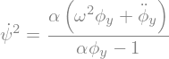
rel1 = sp.solve(eq1,psip**2)[0]
display(sp.Eq(psip**2,rel1))

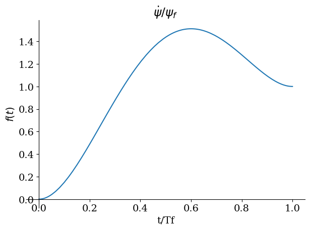
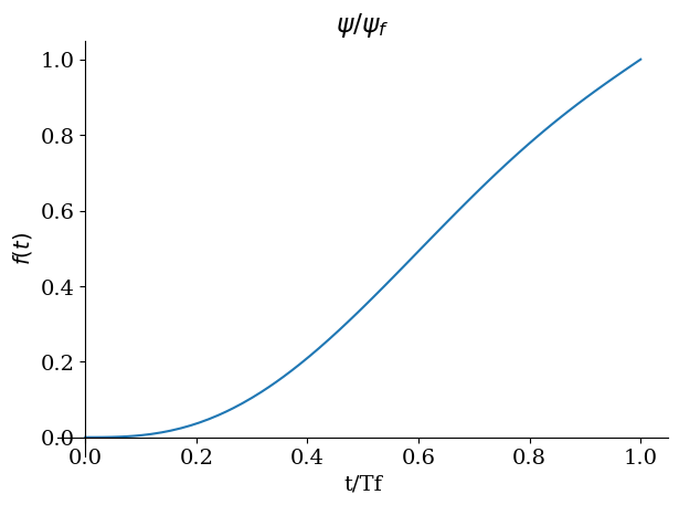
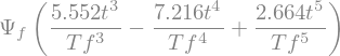
../../_images/1dcb2586d79ac272bc1610eac5f9093ef85f142ad33cdaefed1572c64746e393.png

5.9.1. trajectoire optimale#

on veut choisir $\Psi(t)$ qui assure l’oscillation la plus faible

On détermine le polynôme de degré 5 sans dimension tq: $$\Xi(0)= 0, \frac{d\Xi}{dt}(0)=0, \frac{d^2\Xi}{dt^2}(0)=0$$\Xi(1)= 1, \frac{d\Xi}{dt}(1)=\beta, \frac{d^2\Xi}{dt^2}(1)=0$$

a0,a1,a2,a3,a4,a5 = sp.symbols("a_0 a_1 a_2 a_3 a_4 a_5")
Poly = sp.Lambda(t, a3*t**3 + a4*t**4 + a5*t**5)
Poly(0),Poly(t).diff(t,1).subs(t,0),Poly(t).diff(t,2).subs(t,0)

../../_images/68a3d69cf49ab6e589c4a8fede1a12c1d97a64321b657cc30348a243e19d5865.png

# equations
beta = sp.symbols('beta')
eqs = [Poly(1)-1, Poly(t).diff(t,1).subs(t,1) - beta, Poly(t).diff(t,2).subs(t,1)]
eqs

../../_images/ff2ca3e65d0def3c19ef6c0be387451a17fc64b402b8cf8dac98c2209f6d2b88.png

# solution
coeff = list(sp.linsolve(eqs,[a3,a4,a5]))[0]
coeff

../../_images/f8cb12754615674f65eef1d750971e2b34f29582b295b4c8d02cb70aa7514bad.png

Xi = sp.Lambda(t, coeff[0]*t**3 + coeff[1]*t**4 + coeff[2]*t**5)
display("Xi(t)=",Xi(t))
display("cdts a t=1:",(Xi(1),Xi(t).diff(t,1).subs(t,1),Xi(t).diff(t,2).subs(t,1)))

'Xi(t)='

../../_images/2aea9927ccf1d1c10ac69c346bbfa7fe9ff9ecc6ee667c70a87d2f245b140dd7.png

'cdts a t=1:'

../../_images/7d2267006eea147167cd6b619da638d2dbda689428cea03ad768f72ba3be264f.png

Beta = 1
sp.plot(Xi(t).diff(t).subs(beta,Beta),(t,0,1),title="$\dot{\psi}/\psi_f$",xlabel="t/Tf")
sp.plot(Xi(t).subs(beta,Beta),(t,0,1),title="$\psi/\psi_f$",xlabel="t/Tf");

../../_images/bf2363d2155b6ee68209cafaad19a02cf4f10d180866c2cdc1af1fb538cb1253.png

../../_images/3816d54e500d4d5f2c31c84c519f72750073a07fcf2b0c6e89581a41bac04322.png

5.9.2. Simulation avec psi imposé#

pour déterminer la valeur optimale de $\beta$
définition d’une fonction qui calcule la solution numérique fct de beta
calcul d’un critère: en fin de trajectoire valeur $\phi_y(T)$ et $\dot{\phi_y}(T)$
oscillation: $$ \phi(t) = A \cos(\omega t + \Psi) \mbox{ avec } A cos\psi = \phi_y(T) , -A\omega\sin\psi = \dot{\phi_y}(T)$$ d'où l'amplitude A: $$ A^2 \omega^2 = \omega^2 (\phi_y(T))^2 + (\dot{\phi_y}(T))^2 $$ et l'ordre de grandeur du deplacement max $\approx L A$

Err = lambda Phiy, Phiyp : LL*np.sqrt(Phiy**2 + Phiyp**2/Omega**2)

def solution(Beta,debug=False):
    # calcul Psi
    Psi  = Psif*Xi(t/Tf).subs(beta,Beta)
    if debug: display("Psi=",Psi)
    # calcul lagrangien
    LLa = (La.subs({theta:0,thetap:0, psi: Psi, psip : Psi.diff(t), phiz:0, phizp:0 })).simplify()
    if debug: display("La=",LLa)
    # equation de Lagrange
    LLM = LagrangesMethod(LLa,[phiy])
    Eq = LLM.form_lagranges_equations()
    if debug: display(Eq)
    # transformation EDO dY/dt = F(Y)
    A=LLM.mass_matrix_full
    B=LLM.forcing_full
    FY = A.inv()*B
    FY[1] = FY[1].simplify()
    if debug: display("FY=",FY)
    # fonction python BY
    smBY = sp.lambdify((phiy,phiyp,t,alpha,omega,Psif,Tf),FY,'numpy')
    # fonction F(Y)
    def F(Y,t):
        '''second membre EDO dY/dt = F(Y) avec Y=[phiy,phiyp]'''
        global Alpha,Omega,PsiF,T
        FF =smBY(Y[0],Y[1],t,Alpha,Omega,PsiF,T)
        return FF[:,0]
    # solution numerique
    if debug: print("parametres numerique:",Alpha,Omega,PsiF,T)
    Y0 = np.array([0.,0.])
    N  = 200
    tt = np.linspace(0,T,N)
    sol = odeint(F,Y0,tt)
    PHIY = sol[:,0]
    PHIZ = np.zeros(tt.size)
    PSi  = sp.lambdify(t,Psi.subs({Tf:T,Psif:PsiF}),'numpy')
    PSI  = PSi(tt)
    err  = Err(sol[-1,0],sol[-1,1])
    if debug: print("Erreur: ",err)
    return tt,PSI,PHIY,PHIZ,err

# simulation (val opt 1.14)
Beta = 1.0
tt, PSI, PHIY, PHIZ, err  = solution(Beta,True)

'Psi='

../../_images/b9fbd376577308a03393ff222109c06ca5a5eb93b0549283be6fc1665f306c69.png

'La='

../../_images/459373a95517e862d705b5044fc3ed4443534dad516d15e7c3a31ba6f616e31d.png

../../_images/611687d0b64bb5424532ac7797140caeb355a0c8a349d93d143b702a2fb4da8a.png

'FY='

../../_images/931e1515ffd49d328cdfd15f06cced9a4641c32f3287918d838ebbf800843443.png

parametres numerique: 1.0 2.23606797749979 3.141592653589793 5.0
Erreur:  0.1224537525041114

plt.figure(figsize=(12,8))
plt.subplot(2,1,1)
plt.plot(tt,PHIY,label='$\\phi_y$')
plt.plot(tt,PHIZ,label='$\\phi_z$')
plt.legend()
plt.subplot(2,1,2)
plt.plot(tt,PSI,label="$\psi$")
plt.xlabel('t')
plt.legend();

../../_images/aaa866f4aa3ec52bc1d5e1baf0a9172bdeaf106947ec526b515cebe94f335c09.png

# position de P2
P2X = P2x(0.,PSI,LL)
P2Y = P2y(0.,PSI,LL)
P2Z = P2z(0.,PSI,LL,HH)*np.ones(PSI.size)
# et de M
MX = Mx(0.,PSI,PHIY,PHIZ,LL,Alpha)
MY = My(0.,PSI,PHIY,PHIZ,LL,Alpha)
MZ = Mz(0.,PSI,PHIY,PHIZ,LL,HH,Alpha)
print("Ecart final:",MX[-1]-P2X[-1])

Ecart final: 0.10747021546826074

plt.title("trajectoire dans le plan")
plt.plot(MX,MY,label="M")
plt.plot(P2X,P2Y,label="P2")
plt.xlabel('x')
plt.ylabel('y')
plt.legend()
plt.axis('equal');

../../_images/f1534d11ef6201ae32081fa8ed0f51bc762a8541b53c2d9db37e31fdf1d566dc.png

# etude de l'ecart en fct de beta
BETA  = np.linspace(1,1.2,11)
ECART = np.zeros(BETA.size)
for k in range(BETA.size):
    tt, PSI, PHIY, PHIZ, err = solution(BETA[k])
    ECART[k]=err
    print("beta={:.3f} Ecart final={:.3f}".format(BETA[k],ECART[k]))

beta=1.000 Ecart final=0.122

beta=1.020 Ecart final=0.111

beta=1.040 Ecart final=0.101

beta=1.060 Ecart final=0.093

beta=1.080 Ecart final=0.087

beta=1.100 Ecart final=0.083

beta=1.120 Ecart final=0.083

beta=1.140 Ecart final=0.086

beta=1.160 Ecart final=0.092

beta=1.180 Ecart final=0.100

beta=1.200 Ecart final=0.111

plt.plot(BETA,ECART,'-o')
plt.plot(BETA,np.zeros(BETA.size),'--')
plt.xlabel("$\\beta$")
plt.title("Ecart en fin de trajectoire");

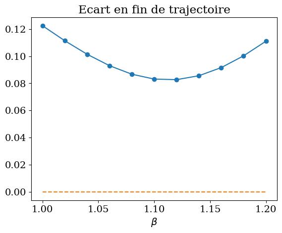
../../_images/f5ec939766f909dc296e9d3be2e3a49081e56800c837e45522d8b532ecf12dad.png

# valeur optimale (minimum)
Bopt = 1.112
print("Bopt={:.4f}".format(Bopt))
# calcul Psi opt
Psi  = Psif*Xi(t/Tf).subs(beta,Bopt)
display("Psi opt=",Psi)

Bopt=1.1120

'Psi opt='

../../_images/5a11e9d0f970e0b92a8dfcc60530fd780f703356155d2ffbe1b7f7a791b7d651.png

5.9.3. Controle avec le couple#

On impose donc un couple $C$ basé sur un régulateur simple pour obtenir la trajectoire $\psi_i(t)$ imposée

\[ C_c = -K_c \left( (\psi-\psi_i) + T_c(\dot{\psi}-\dot{\psi_i})\right) \]

Kc, Tc = sp.symbols('K_c T_c')
Cc = -Kc*((psi-Psi)+(psip-Psi.diff(t,1))*Tc)
display("Couple C=",Cc)

'Couple C='

../../_images/7fbd912d35d62250e33a538fbf6454c24524c7c8d6a498a4341e6516cb333f64.png

C = sp.symbols('C')
LLa = La.subs({theta:0,thetap:0, phiz:0, phizp:0 }).simplify()
display("Lagrangien:",LLa)
LLM = LagrangesMethod(LLa,[phiy,psi],forcelist=[(Rb,C*RO.z)],frame=RO)
Eq = LLM.form_lagranges_equations()
display("Equations",Eq)

'Lagrangien:'

'Equations'

../../_images/c1a900a955d187b685428ad1298547dac0ac9d913670b1ce4fca4cbba871daae.png

# transformation EDO dY/dt = F(Y)
A=LLM.mass_matrix_full
B=LLM.forcing_full
FY = A.inv()*B
FY[2]=FY[2].simplify()
FY[3]=FY[3].simplify()
display("FY=",FY)

'FY='

../../_images/3e7818b32ec1af0f03504c3b4988c5cc90a0ed56bc6d5d872a5d684676f43ddd.png

# fonction BY
smBY = sp.lambdify([phiy,psi,phiyp,psip,alpha,omega,C],FY,'numpy')
# et couple
CC   = sp.lambdify([psi,psip,t,Psif,Tf,Kc,Tc],Cc,'numpy')

# fonction F(Y)
def F(Y,t):
    '''second membre EDO dY/dt = F(Y) avec Y=[phiy,psi,phiyp,psip]'''
    global Alpha,Omega,T,PsiF,KC,TC
    Ci = CC(Y[1],Y[3],t,PsiF,T,KC,TC)
    FF =smBY(Y[0],Y[1],Y[2],Y[3],Alpha,Omega,Ci)
    return FF[:,0]

# solution numerique
KC = 100
TC = 800./KC
print("parametres:",Alpha,Omega,PsiF,T,KC,TC)
Y0 = np.array([0.0,0.0,0.,0.])
# avec perturbation en psi
#Y0 = np.array([0.0,0.1,0.,0.])
N  = 200
tt = np.linspace(0,T,N)
sol = odeint(F,Y0,tt)
PHIY = sol[:,0]
PSI  = sol[:,1]
err = Err(sol[-1,0],sol[-1,2])
print("Erreur:",err)

parametres: 1.0 2.23606797749979 3.141592653589793 5.0 100 8.0
Erreur: 0.09357936449364572

plt.figure(figsize=(12,8))
plt.subplot(2,1,1)
plt.plot(tt,PHIY,label='$\\phi_y$')
plt.legend()
plt.subplot(2,1,2)
plt.plot(tt,PSI,label="$\psi$")
plt.xlabel('t')
plt.legend();

../../_images/c015ed6eec9a8b7ba77cd2d316cfb1ad20a135e31e1f81e560d05539a5d28224.png

# position de P2
P2X = P2x(0.,PSI,LL)
P2Y = P2y(0.,PSI,LL)
P2Z = P2z(0.,PSI,LL,HH)*np.ones(PSI.size)
# et de M
MX = Mx(0.,PSI,PHIY,PHIZ,LL,Alpha)
MY = My(0.,PSI,PHIY,PHIZ,LL,Alpha)
MZ = Mz(0.,PSI,PHIY,PHIZ,LL,HH,Alpha)
print("Ecart final:",MX[-1]-P2X[-1])

Ecart final: -0.003938349868875868

plt.title("trajectoire dans le plan")
plt.plot(MX,MY,label="M")
plt.plot(P2X,P2Y,label="P2")
plt.xlabel('x')
plt.ylabel('y')
plt.legend()
plt.axis('equal');

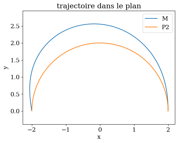
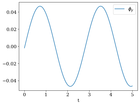
../../_images/ac5187cc4fdb7f607cb5b9c4d9ebfbeb3bd914d5fa93271fc661e4d381e57c70.png

5.10. oscillation en fin de trajectoire#

# resolution numérique
Y0f = sol[-1,::2]
print(Y0f)
ttf  = np.linspace(T,2*T,N)
solf = odeint(Ff,Y0f,ttf)
PHIYf = solf[:,0]
PHIZf = np.zeros(ttf.size)

[-0.00196919  0.10453221]

plt.plot(tt,PHIYf,label='$\\phi_y$')
plt.legend()
plt.xlabel('t');

../../_images/6f8bc8de1589e62e00f663f21976a050c02d47fd252ee3b4ff8748cb29757b58.png

# position de P2 et M
P2X = P2x(0.,PsiF,LL)*np.ones(PHIYf.size)
P2Y = P2y(0.,PsiF,LL)*np.ones(PHIYf.size)
P2Z = P2z(0.,PsiF,LL,HH)*np.ones(PHIYf.size)
MX = Mx(0.,PsiF,PHIYf,PHIZf,LL,Alpha)
MY = My(0.,PsiF,PHIYf,PHIZf,LL,Alpha)
MZ = Mz(0.,PsiF,PHIYf,PHIZf,LL,HH,Alpha)

plt.plot(MX,MY)
plt.plot(MX[0],MY[0],'x')
plt.plot(P2X,P2Y,'o')
plt.title("Trajectoire plan")
plt.axis('equal');

../../_images/771f758df31bab835b13c5d5197a3fb59e384f9bcc0fe4dc8540853193f1b566.png