5. Modèles d’équations

A partir des équations générales de la mécanique des fluides d’un écoulement monophasique, on va passer en revu différents modèles classiques d’équations en mécanique des fluide, en

• décrivant rapidement les différentes approximations

• discutant rapidement les domaines d’application

Opérateurs:

Pour obtenir ces équations, on utilise les propriétés d’analyse vectorielle suivantes:

\[div(\overrightarrow{grad}\,u)=\Delta u,\,\,\,\,\overrightarrow{rot}(\overrightarrow{grad}\,u)=0\]

\[\overrightarrow{rot}(\overrightarrow{U}\otimes\overline{\overline{grad}}\,\overrightarrow{U})=\overrightarrow{U}\otimes\overline{\overline{grad}}(\overrightarrow{rot}(\overrightarrow{U}))+rot(\overrightarrow{U})*div(\overrightarrow{U})\]

5.1. Écoulement de Stokes

cas limite \(Re \rightarrow 0\)

Modèle écoulement incompressible visqueux de Stokes (\(p=p'+P_{0}\))

\[\begin{split}\begin{aligned} div\,\overrightarrow{U} & =0\\ -\overrightarrow{grad}\left(p^{'}\right)+\mu\Delta\overrightarrow{U} & =0\end{aligned}\end{split}\]

exemple: écoulement d’huile dans un tuyau horizontal \(L=0.15m\) de rayon \(R=2mm\) débit \(Q=0.02\,l/min\) (\(U_{0}=0.03m/s)\)

huile moteur liquide incompressible: \(\rho=860\,kg/m^{3}\) et \(\mu=0.2\,Pa.s\)

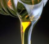
Fig. 5.1 écoulement d’huile

5.2. Fluide parfait incompressible

cas limite \(Re=\infty\) , \(Ma\ll1\)

Modèle écoulement fluide parfait incompressible

\[\begin{split}\begin{aligned} div\,\overrightarrow{U} & =0\\ \frac{D\overrightarrow{U}}{Dt}& =-\overrightarrow{\nabla}(\frac{p}{\rho}+gz) \end{aligned} \end{split}\]

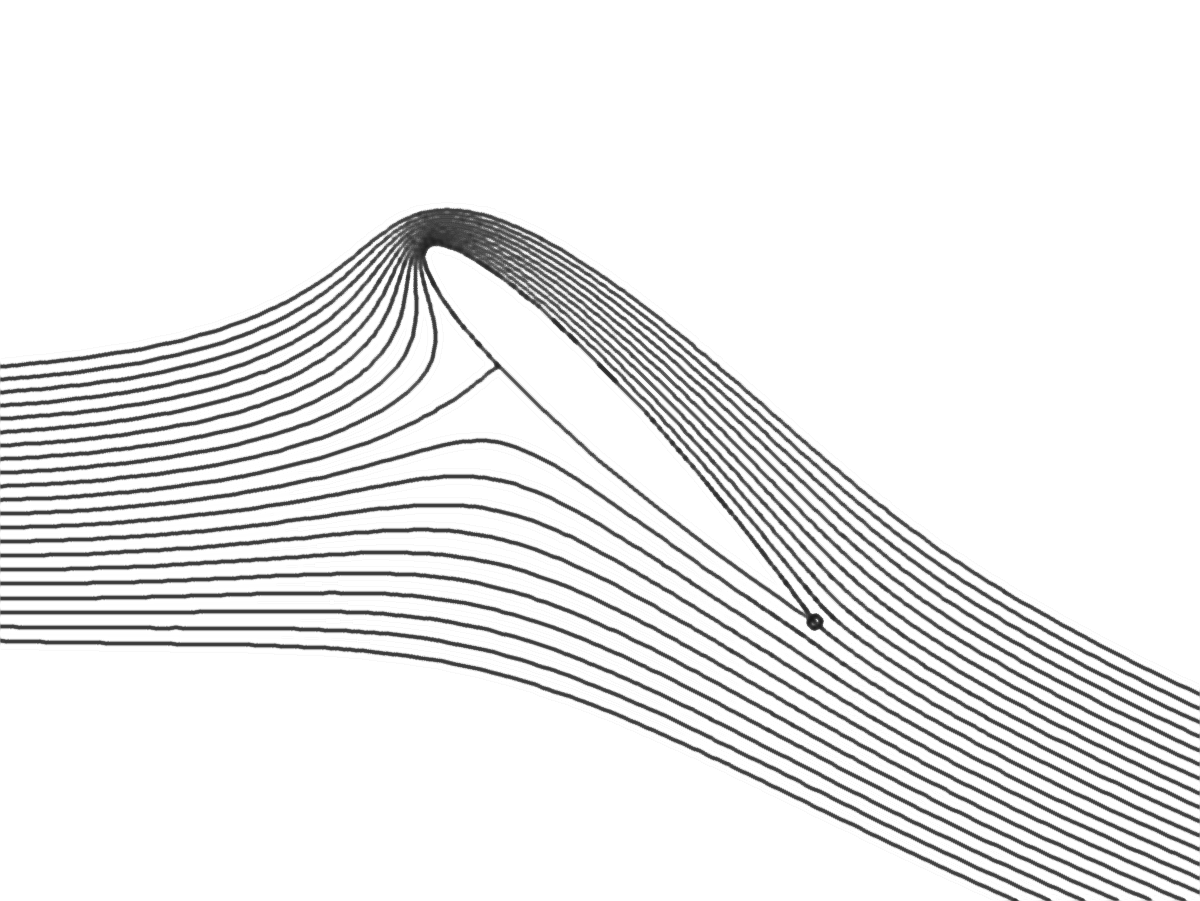
Fig. 5.2 écoulement autour d’un profil d’aile

Pour un champ de vitesse \(\overrightarrow{U}\), on définit sa circulation \(\Gamma\) le long d” un contour fermé \(C\) par:

\[\Gamma=\oint_{c}\overrightarrow{U}.\overrightarrow{dl}\]

En utilisant le théoréme du rotationnel, \(\Gamma\) s’exprime en fonction du flux du rotationnel à travers la surface \(S\) limité par \(C\)

\[\Gamma = \iint_{S}rot\overrightarrow{U}.\overrightarrow{n}\,ds \]

En prenant le rotationnel de l’équation de bilan de quantité de mouvement et en notant que \(\overrightarrow{rot}(\overrightarrow{grad}(\;))=0\),on montre le théorème suivant:

théorème de Kelvin: pour un fluide parfait incompressible, on a conservation de la circulation le long de tout contour fermé $\(\frac{D\Gamma}{Dt}=0\Longleftrightarrow\frac{D}{Dt}\left(\iint_{S}rot\overrightarrow{u}.\overrightarrow{n}\,ds\right)=0\)$

On en déduit qu’un fluide parfait irrotationnelle à \(t=0\) reste irrotationnelle \(\overrightarrow{\omega}=rot\overrightarrow{u}=\overrightarrow{0}\).

Un champ de vitesse irrotationnel découle d’un potentiel $\(rot\overrightarrow{U}=0\,\Longrightarrow\overrightarrow{U}=\overrightarrow{grad}(\Phi)\)$

ce qui pour un fluide incompressible conduit à

\[div\overrightarrow{U}=0\,\Longrightarrow\Delta\Phi=0\]

Modèle d’écoulement potentiel

L’écoulement d’un fluide parfait incompressible irrotationnel est un écoulement potentiel solution de $\(\Delta\Phi=0\)$

En 2D, on peut remplacer le potentiel \(\phi\) par fonction de courant \(\psi\), qui vérifie aussi une équation de Laplace:

\[\Delta\psi=0\]

On peut alors étudier les écoulements potentiels en 2D en utilisant les outils de l’analyse complexe en introduisant le potentiel complexe \(\Psi(z) = \phi(x,y) +i \, \psi(x,y)\) qui est une fonction holomorphe.

Mais attention aux conditions aux limites!!

5.3. Écoulement incompressible isotherme

cas \(Re\gg 1\) , \(Ma\ll 1\)

Équations classiques de Navier-Stokes

5.3.1. Écoulement incompressible avec effet de gravité

\[\begin{split}\begin{aligned} div\,\overrightarrow{U} & =0\\ \rho_{0}\frac{\partial\overrightarrow{U}}{\partial t}+\rho_{0}\overrightarrow{U}.\overrightarrow{grad}\,\overrightarrow{U} & =-\overrightarrow{grad}\left(p'+\rho_{0}gz\right)+\mu\Delta\overrightarrow{U}\end{aligned}\end{split}\]

**exemple ** écoulement d’eau dans conduite forcée de diamètre \(D=1m\) ayant une chute de \(L=85m\) avec un débit \(Q=3\,m^{3}/s\) (\(U_{0}=3.8\,m/s)\)

eau liquide incompressible : \(\rho=1000\,kg/m^{3}\) et \(\mu=10^{-3}\,Pa.s\)

\(Re=3.8\,10^{6},\,\,Fr=0.13\)

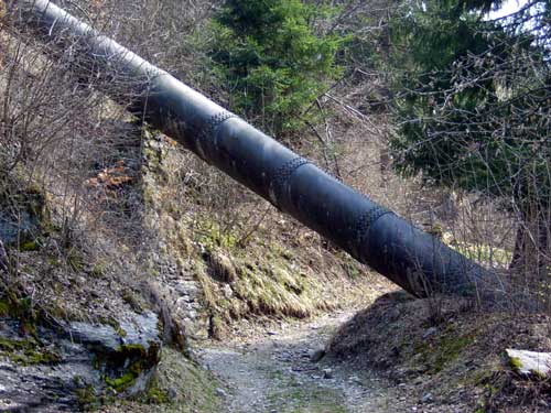
Fig. 5.3 écoulement dans une conduite forcée

5.3.2. Écoulement incompressible de Navier-Stokes

En notant \(\nu=\mu/\rho_{0}\) la viscosité cinématique

\[\begin{split}\begin{aligned} div\,\overrightarrow{U} & =0\\ \frac{\partial\overrightarrow{U}}{\partial t}+\overrightarrow{U}.\overrightarrow{grad}\,\overrightarrow{U} & =-\overrightarrow{grad}p'+\nu\Delta\overrightarrow{U}\end{aligned}\end{split}\]

**exemple **: écoulement d’air autour d’une voiture à \(90km/h\) \((U_{0}=25\,m/s)\) avec \(H=1.5m\)

fluide air: \(\rho=1kg/m^{3}\) et \(\mu=15\,10^{-6}\,Pa.s\) et \(c_{0}=330\,m/s\)

\(Re=2.5\,10^{6}\) et \(Ma=0.07\)

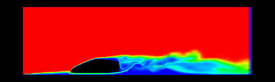
Fig. 5.4 écoulement autour d’une voiture

5.4. Approximation de Boussinesq

cas d’écoulement atmosphérique \(Re\gg 1\) , \(Ma\ll 1\)

avec prise en compte de

1. variation de la masse volumique (linéarisation) $\(\rho=\rho(T)=\rho_{0}-\beta\theta \mbox{ avec } \beta=\rho_{0}/T_{0} \mbox{ et } \theta=T-T_{0}\)$

2. rotation de la terre\(\Longrightarrow\) effet de Coriolis + effet centrifuge

\[\begin{split}\begin{aligned} div\,\overrightarrow{U} & =0\\ \rho_{0}\left(\frac{\partial\overrightarrow{U}}{\partial t}+\overrightarrow{U}.\overrightarrow{grad}\,\overrightarrow{U}+2\overrightarrow{\Omega}\wedge\overrightarrow{U}+\overrightarrow{\Omega}\wedge\overrightarrow{\Omega}\wedge\overrightarrow{r}\right) & =-\overrightarrow{grad}\left(p'+\rho_{0}gz\right)\\ & +\beta\theta+\mu\Delta\overrightarrow{U}\\ \rho_{0}C_{p}\frac{\partial\theta}{\partial t}+\rho_{0}\overrightarrow{U}.\overrightarrow{grad}\,\theta & =\lambda\Delta\theta\end{aligned}\end{split}\]

exemple écoulement atmosphérique

• Richardson \(Ri\sim 1/Fr^{2}\) (caractérise l’effet de la variation de température sur la dynamique et la stabilité)

• échelle \(h \gg km\) vitesse \(u\sim0-100km/h\)

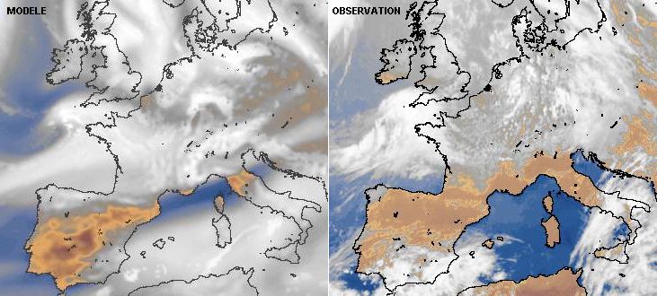
Fig. 5.5 écoulement en météorologie

5.5. Écoulement compressible

cas d’écoulement avec effet de compressibilité \(Re=\infty\)

Modèle: fluide parfait compressible

5.5.1. Équations d’Euler

\[\frac{\partial\rho}{\partial t}+div(\rho\overrightarrow{U})=0\]

\[\frac{\partial\rho\overrightarrow{U}}{\partial t}+div(\rho\overrightarrow{U}\otimes\overrightarrow{U})=-\overrightarrow{grad}\,p\]

\[\frac{\partial\rho(e+\frac{1}{2}V^{2})}{\partial t}+div((\rho(e+\frac{1}{2}V^{2})+p)\overrightarrow{U})=0\]

\[\mbox{ avec } e=\frac{1}{\gamma-1}\frac{p}{\rho}\]

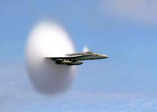
Fig. 5.6 Ondes de choc autour d’un F18

5.5.2. Acoustique

En considérant de petites fluctuations de masse volumique \(\rho'\), de pression \(p'\) et de vitesse \(U'\) autour d’un état de base au repos \(\rho_0\) et \(p_0\), les champs de \(\rho=\rho_{0}+\rho'\), \(p=p_{0}+p'\), \(\overrightarrow{U} = \overrightarrow{U'}\) vérifient les équation d’Euler.

En linéarisant autour de cet état de base, on pour obtenir:

\[\begin{split}\begin{aligned} \frac{\partial\rho'}{\partial t}+div(\rho_{0}\overrightarrow{U}') & =0\\ \frac{\partial\rho_{0}\overrightarrow{U'}}{\partial t} & =-\overrightarrow{grad}\,p'\\ \frac{p'}{p_{0}}-\gamma\frac{\rho'}{\rho_{0}} & =0\end{aligned}\end{split}\]

ce qui conduit à l” équations de propagation d’ondes sonores

\[\frac{\partial^{2}p}{\partial t^{2}}-\gamma\frac{p_{0}}{\rho_{0}}\Delta p=0\]

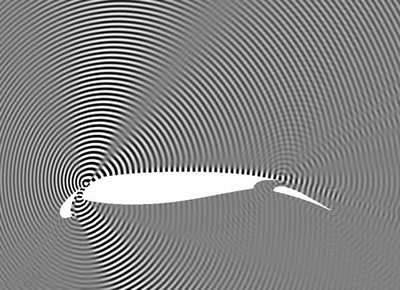
Fig. 5.7 Propagation d’ondes sonores autour d’un profil à 3 corps