4.5. Ondes de gravité et surface libre

Marc BUFFAT, département mécanique Lyon 1

%matplotlib inline
import numpy as np
import scipy as sp
import matplotlib.pyplot as plt
from IPython.core.display import HTML
import matplotlib.animation as animation
from matplotlib import rc
from metakernel import register_ipython_magics
register_ipython_magics()

from IPython.display import YouTubeVideo

YouTubeVideo('MNyebpog_i0', width=600, height=400)

4.5.1. Equation des ondes de surface

soit \(h(x,t)\) la variation de la hauteur d’eau dans un bassin de longueur \(L\) et \(u(x,t)\) la perturbation de vitesse horizontale. Les équations de SAint Venant linéarisées s’écrivent:

• bilan de masse:

\[ \frac{\partial h}{\partial t} + h_0 \frac{\partial u}{\partial x} = 0 \]

• bilan de qte mouvement horizontal

\[ h_0\frac{\partial u}{\partial t} + g h_0 \frac{\partial h}{\partial x} = 0 \]

Il peut se développer des ondes de surface dans un bassin de longueur L, solution de l’équation des ondes:

\[\frac{\partial^2 h}{\partial t^2} - c_0^2\frac{\partial^2h}{\partial x^2}=0\]

avec des conditions aux limites \(\frac{\partial h}{\partial x}(0,t) = \frac{\partial h}{\partial x}(L,t) = 0\) :

• solution élémentaire: onde stationnaire $\(hk(x,t)=A_{k}\cos(\frac{k\pi x}{L})\cos(\frac{k\pi c_{0}t}{L})\)$

• solution générale $\(h'(x,t)=\sum_{k}A_{k}\cos(\frac{k\pi x}{L})\cos(\frac{k\pi c_{0}t}{L})\)$

4.5.1.1. paramètres

• g gravité

• h0 hauteur d’eau

• a0 amplitude perturbation

• L longueur bassin

Influences des paramètres sur le mouvement des ondes ?

# parametres
g=10.0
h0=1.
a0=0.1
c0=np.sqrt(g*h0)
L =20.
Np=128
X=np.linspace(0,L,Np,endpoint=False)
print("parametres célérité= {:.2f}m/s   h0/L={:.3f}  a0/h0={:.3f}".format(c0,h0/L,a0/h0))

parametres célérité= 3.16m/s   h0/L=0.050  a0/h0=0.100

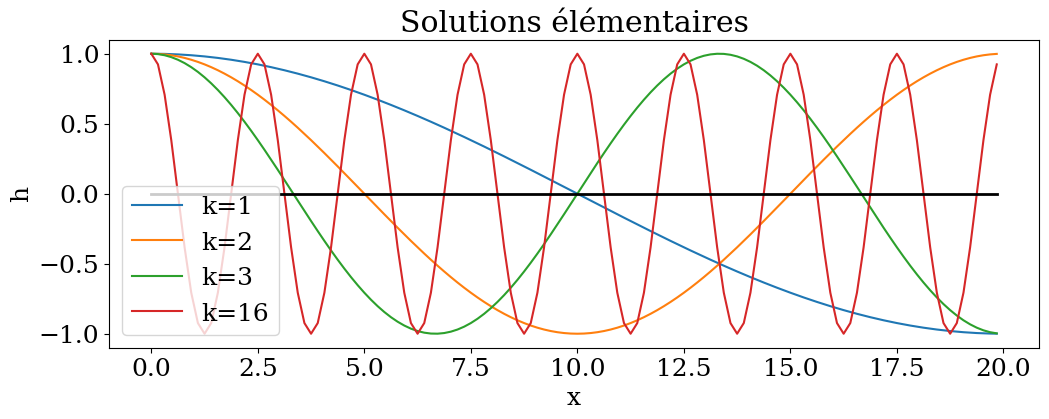
4.5.1.2. solution élémentaire: onde stationnaire

# solution elementaire CL de tye Neuman
def hk(k,x,t):
    global c0,L
    return np.cos(k*np.pi*x/L)*np.cos(k*np.pi*c0*t/L)

# solutions elementaires
plt.rc('font', family='serif', size='18')
plt.figure(figsize=(12,4))
plt.plot(X,hk(1,X,0),label="k=1")
plt.plot(X,hk(2,X,0),label="k=2")
plt.plot(X,hk(3,X,0),label="k=3")
plt.plot(X,hk(16,X,0),label="k=16")
plt.plot(X,np.zeros(X.size),'-k',lw=2)
plt.legend()
plt.title("Solutions élémentaires")
plt.xlabel('x')
plt.ylabel('h');

#%activity /usr/local/commun/ACTIVITY/MGC3062L/questionOndeStationnaire

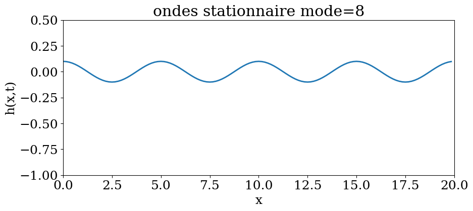
4.5.1.2.1. animation

# choix du mode
mode=8
#
periode=2*L/(mode*c0)
t=np.linspace(0,2*periode,41)
fig = plt.figure(figsize=(10,4))      
ax  = plt.axes()
line, = ax.plot([], [],linewidth=2)  
plt.axis((0,L,-1.,0.5))
plt.title("ondes stationnaire mode={}".format(mode))
plt.xlabel('x')
plt.ylabel('h(x,t)')
def plot_mode(t):
    Y = a0*hk(mode,X,t)
    line.set_data(X,Y) 
    
anim=animation.FuncAnimation(fig, plot_mode, frames=t)

rc('animation', html='jshtml')
anim

Once Loop Reflect

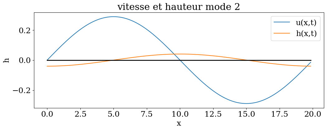
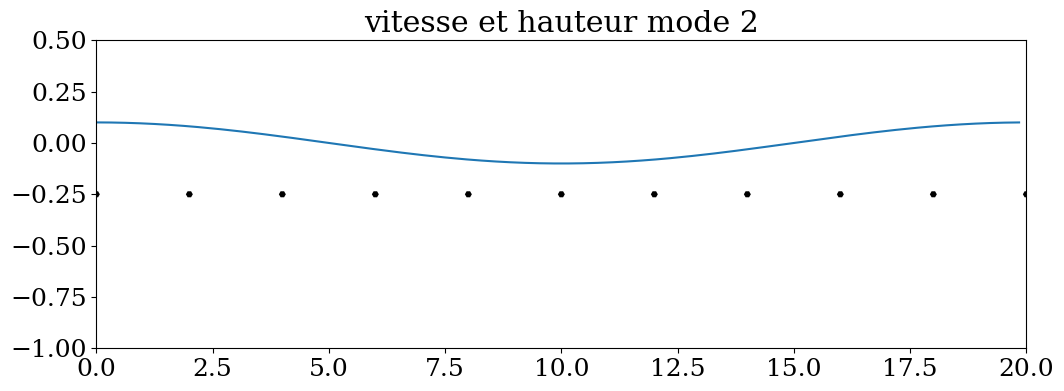
4.5.1.3. calcul de la vitesse u(x,t)

\[ \frac{\partial u}{\partial t} + g\frac{\partial h}{\partial x} = 0\]

def uk(k,x,t):
    global c0,L,g
    return (g/c0)*np.sin(k*np.pi*x/L)*np.sin(k*np.pi*c0*t/L)

mode=2
plt.figure(figsize=(12,4))
plt.plot(X,a0*uk(mode,X,2),label="u(x,t)")
plt.plot(X,a0*hk(mode,X,2),label="h(x,t)")
plt.plot(X,np.zeros(X.size),'-k',lw=2)
plt.legend()
plt.title("vitesse et hauteur mode {}".format(mode))
plt.xlabel('x')
plt.ylabel('h');

4.5.1.3.1. Animation

mode = 2
periode=2*L/(mode*c0)
t=np.linspace(0,2*periode,41)
XP = np.linspace(0,L,11)
YP = -0.25*np.ones(XP.size)
UP = a0*uk(mode,XP,0)+1.e-3
VP = np.zeros(UP.size)
fig = plt.figure(figsize=(12,4))
ax  = plt.axes()
plt.axis((0,L,-1.,0.5))
Q   = ax.quiver(XP,YP,UP,VP,scale_units='xy',scale=0.1)
Line, = plt.plot(X,a0*hk(mode,X,2),label="h(x,t)")
plt.title("vitesse et hauteur mode {}".format(mode))
def plot_mode(t):
    Y  = a0*hk(mode,X,t)
    Line.set_data(X,Y)
    UP = a0*uk(mode,XP,t)+1.e-3
    Q.set_UVC(UP,VP)
#
anim=animation.FuncAnimation(fig, plot_mode, frames=t)

rc('animation', html='jshtml')
anim

Once Loop Reflect

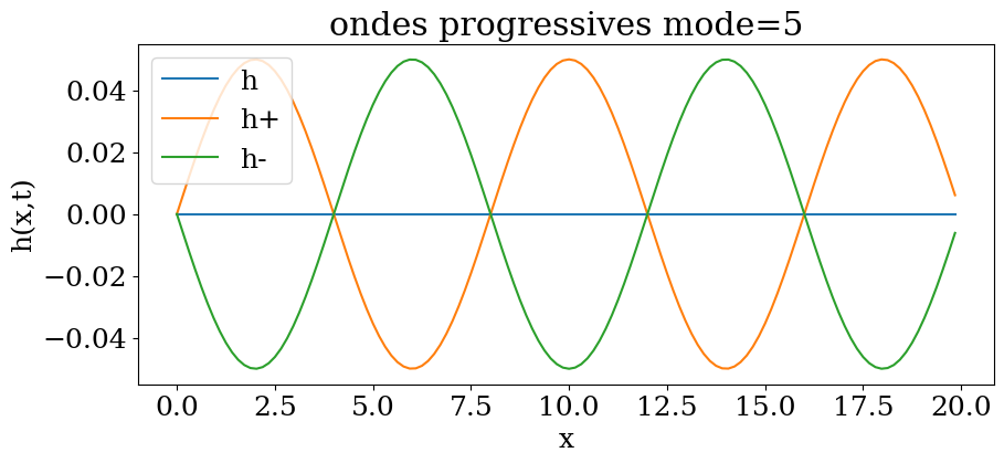
4.5.1.4. décomposition en ondes progressives

utilisation de l’identité trigonométrique

\[ \cos a \cos b = \frac{1}{2} (\cos(a+b) + \cos(a-b))\]

# ondes progressive et régressive
def hkp(k,x,t):
    global c0,L
    return 0.5*np.cos(k*np.pi*(x-c0*t)/L)
def hkm(k,x,t):
    global c0,L
    return 0.5*np.cos(k*np.pi*(x+c0*t)/L)

mode = 5
t0 = 2*L/(mode*c0)/4
plt.figure(figsize=(10,4))
plt.title("ondes progressives mode={}".format(mode))
plt.xlabel('x')
plt.ylabel('h(x,t)')
plt.plot(X,a0*hk(mode,X,t0),label="h")
plt.plot(X,a0*hkp(mode,X,t0),label="h+")
plt.plot(X,a0*hkm(mode,X,t0),label="h-")
plt.legend();

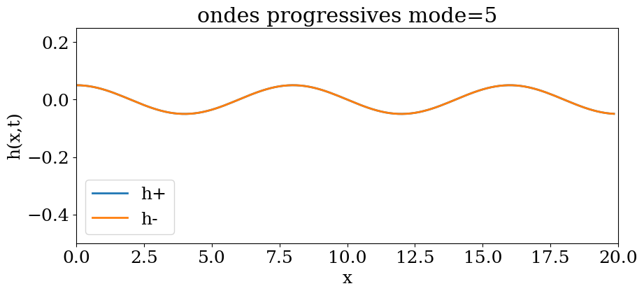
4.5.1.4.1. Animation

periode=2*L/(mode*c0)
t=np.linspace(0,2*periode,41)
fig = plt.figure(figsize=(10,4))      
ax  = plt.axes()
line1, = ax.plot([], [],linewidth=2,label="h+") 
line2, = ax.plot([], [],linewidth=2,label="h-") 
plt.axis((0,L,-0.5,0.25))
plt.title("ondes progressives mode={}".format(mode))
plt.xlabel('x')
plt.ylabel('h(x,t)')
plt.legend()
def plot_mode(t):
    Y1 = a0*hkp(mode,X,t)
    line1.set_data(X,Y1)
    Y2 = a0*hkm(mode,X,t)
    line2.set_data(X,Y2)
    return
anim=animation.FuncAnimation(fig, plot_mode, frames=t)

rc('animation', html='jshtml')
anim

Once Loop Reflect

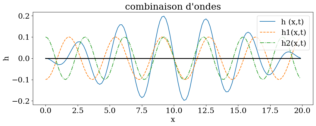
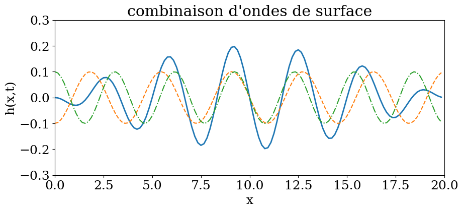
4.5.1.5. combinaison d’ondes stationnaires

mode = 12
combi = lambda x,t : (-hk(mode-1,x,t)+hk(mode+1,x,t))*a0
onde1 = lambda x,t : (-hk(mode-1,x,t))*a0
onde2 = lambda x,t : ( hk(mode+1,x,t))*a0

plt.figure(figsize=(12,4))
plt.plot(X,combi(X,0),label="h (x,t)")
plt.plot(X,onde1(X,0),'--',label="h1(x,t)")
plt.plot(X,onde2(X,0),'-.',label="h2(x,t)")
plt.plot(X,np.zeros(X.size),'-k',lw=2)
plt.legend()
plt.title("combinaison d'ondes")
plt.xlabel('x')
plt.ylabel('h');

4.5.1.5.1. animation

# solution générale: combinaison de solutions elemetaires
periode=2*L/(mode*c0)
t=np.linspace(0,4*periode,80)
fig = plt.figure(figsize=(10,4))      
ax  = plt.axes()
line, = ax.plot([], [],linewidth=2)  
line1, = ax.plot([], [],'--')  
line2, = ax.plot([], [],'-.')  

plt.axis((0,L,-0.3,0.3))
plt.title("combinaison d'ondes de surface")
plt.xlabel('x')
plt.ylabel('h(x,t)')
def plot_mode(t):
    Y = combi(X,t)
    line.set_data(X,Y) 
    Y1 = onde1(X,t)
    line1.set_data(X,Y1)
    Y2 = onde2(X,t)
    line2.set_data(X,Y2)
anim=animation.FuncAnimation(fig, plot_mode, frames=t)

rc('animation', html='jshtml')
anim

Once Loop Reflect

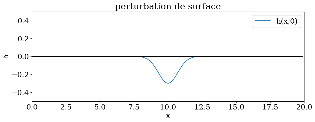
4.5.1.6. cas générale: décomposition en série

# perturbation initiale
hp=lambda x:-3*a0*np.exp(-(x-L/2)**2/1**2)

plt.figure(figsize=(12,4))
plt.plot(X,hp(X),label="h(x,0)")
plt.plot(X,np.zeros(X.size),'-k',lw=2)
plt.axis((0,L,-0.5,0.5))
plt.legend()
plt.title("perturbation de surface")
plt.xlabel('x')
plt.ylabel('h');

%activity /usr/local/commun/ACTIVITY/MGC3062L/questionPerturbation

Error in calling magic 'activity' on line:
    [Errno 2] No such file or directory: '/usr/local/commun/ACTIVITY/MGC3062L/questionPerturbation'
    args: ['/usr/local/commun/ACTIVITY/MGC3062L/questionPerturbation']
    kwargs: {}
Traceback (most recent call last):
  File "/home/buffat/venvs/jupyter/lib/python3.10/site-packages/metakernel/magic.py", line 96, in call_magic
    func(*args, **kwargs)
  File "/home/buffat/venvs/jupyter/lib/python3.10/site-packages/metakernel/magics/activity_magic.py", line 265, in line_activity
    activity.load(filename)
  File "/home/buffat/venvs/jupyter/lib/python3.10/site-packages/metakernel/magics/activity_magic.py", line 31, in load
    with open(self.filename) as fp:
FileNotFoundError: [Errno 2] No such file or directory: '/usr/local/commun/ACTIVITY/MGC3062L/questionPerturbation'

%activity FILENAME - run a widget-based activity
  (poll, classroom response, clicker-like activity)

This magic will load the JSON in the filename.

Examples:
    %activity /home/teacher/activity1
    %activity /home/teacher/activity1 new
    %activity /home/teacher/activity1 edit

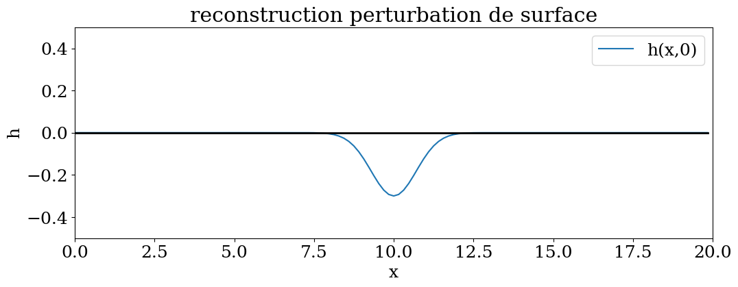
4.5.1.6.1. décomposition en série de Fourier

# calcul FFT de la CI x exp(alpha*X)
from scipy.fftpack import fft, ifft, rfft
HP  = hp(X)
# attention FFT sur un domaine double
HPF = np.zeros(2*Np)
HPF[:Np]= HP[:]
HPF[Np:]= HP[:]
HPS=fft(HPF)

# reconstruction avec nmode
nmode=16
HP1 = np.ones(Np)*HPS[0].real/(2*Np)
for k in range(2,2*nmode,2):
        HP1 += HPS[k].real*hk(k,X,0)/Np
print("amplitude solution=",np.min(HP1),np.max(HP1))

amplitude solution= -0.2998320170193419 0.00010105515111780661

plt.figure(figsize=(12,4))
plt.plot(X,HP1,label="h(x,0)")
plt.plot(X,np.zeros(X.size),'-k',lw=2)
plt.axis((0,L,-0.5,0.5))
plt.legend()
plt.title("reconstruction perturbation de surface")
plt.xlabel('x')
plt.ylabel('h');

# evolution en temps
def solh(x,t):
    sol1 = np.ones(Np)*HPS[0].real/(2*Np)
    for k in range(2,2*nmode,2):
             sol1 += (HPS[k].real/Np)*hk(k,x,t)
    return sol1

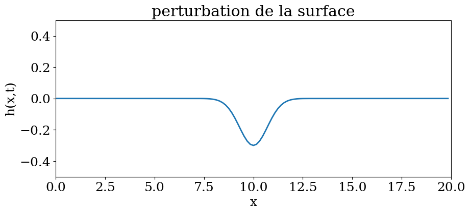
4.5.1.6.2. Animation

# animation
periode=2*L/(mode*c0)
t=np.linspace(0,5*periode,40)
fig = plt.figure(figsize=(10,4))      
ax  = plt.axes()
line, = ax.plot([], [],linewidth=2)  
plt.axis((0,L,-0.5,0.5))
plt.title("perturbation de la surface")
plt.xlabel('x')
plt.ylabel('h(x,t)')
def plot_mode(t):
    line.set_data(X,solh(X,t)) 
    
anim=animation.FuncAnimation(fig, plot_mode, frames=t)

rc('animation', html='jshtml')
anim

Once Loop Reflect

4.5.2. Ondes de surface dispersives

• étude avec une célérité \(c_0\) fonction de la fréquence (ou du mode k)

\[ c(k) = c_0 (1- \frac{k}{50})\]

# loi de célérité
def c0d(k):
    return c0*(1-0.02*k)

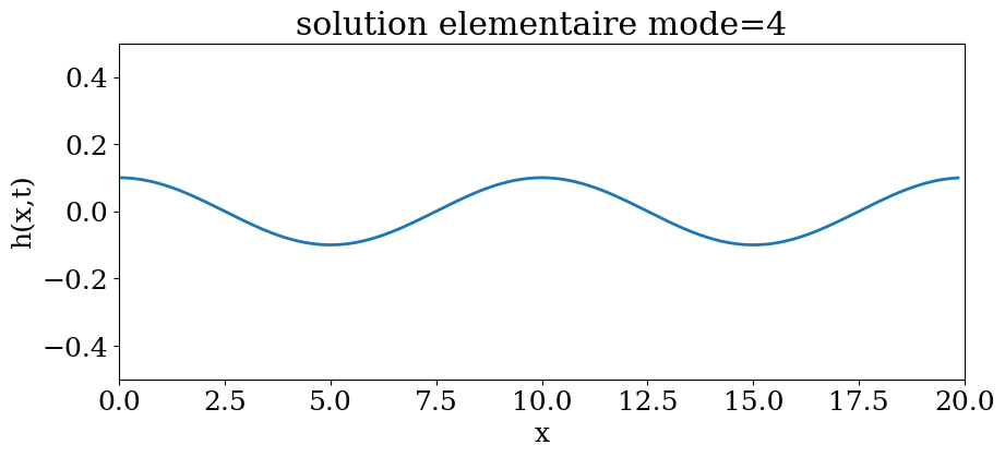
4.5.2.1. solution élémentaire

# solution elemntaire
def hkd(k,x,t):
        return np.cos(k*np.pi*x/L)*np.cos(k*np.pi*c0d(k)*t/L)

4.5.2.1.1. Animation

# solution élémentaire animation
mode=4
periode=2*L/(mode*c0)
t=np.linspace(0,2*periode,20)
fig = plt.figure(figsize=(10,4))      
ax  = plt.axes()
line, = ax.plot([], [],linewidth=2)  
plt.axis((0,L,-0.5,0.5)) 
plt.title("solution elementaire mode={}".format(mode))
plt.xlabel('x')
plt.ylabel('h(x,t)')
def plot_mode(t):
    line.set_data(X,a0*hkd(mode,X,t)) 
    
anim=animation.FuncAnimation(fig, plot_mode, frames=t)

rc('animation', html='jshtml')
anim

Once Loop Reflect

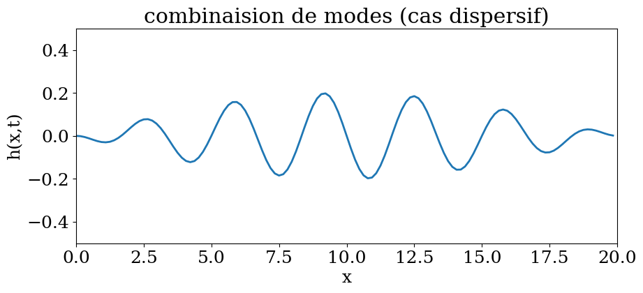
4.5.2.2. combinaison d’ondes stationnaires

mode = 12
combi = lambda x,t : (-hk(mode-1,x,t)+hk(mode+1,x,t))*a0

4.5.2.2.1. animation

# combinaison d'ondes: somme d'ondes
periode=2*L/(mode*c0)
t=np.linspace(0,4*periode,41)
fig = plt.figure(figsize=(10,4))      
ax  = plt.axes()
line, = ax.plot([], [],linewidth=2)  
plt.axis((0,L,-0.5,0.5)) 
plt.title("combinaision de modes (cas dispersif)")
plt.xlabel('x')
plt.ylabel('h(x,t)')
def plot_mode(t):
    line.set_data(X,combi(X,t)) 
    
anim=animation.FuncAnimation(fig, plot_mode, frames=t)

rc('animation', html='jshtml')
anim

Once Loop Reflect

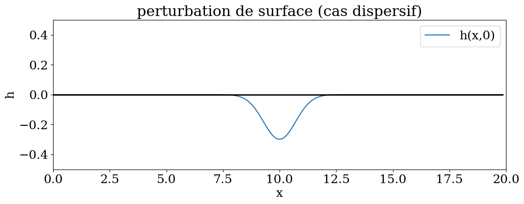
4.5.2.3. cas général: décomposition en serie

# evolution en temps
def solhd(x,t):
    sol1 = np.ones(Np)*HPS[0].real/(2*Np)
    for k in range(2,2*nmode,2):
             sol1 += (HPS[k].real/Np)*hkd(k,x,t)
    return sol1

plt.figure(figsize=(12,4))
plt.plot(X,solhd(X,0),label="h(x,0)")
plt.plot(X,np.zeros(X.size),'-k',lw=2)
plt.axis((0,L,-0.5,0.5))
plt.legend()
plt.title("perturbation de surface (cas dispersif)")
plt.xlabel('x')
plt.ylabel('h');

#%activity /usr/local/commun/ACTIVITY/MGC3062L/questionDispersion

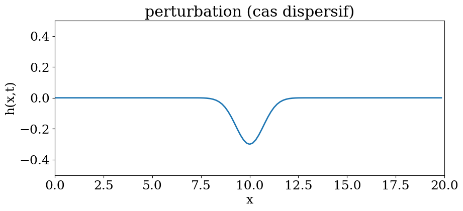
4.5.2.3.1. animation

# animation
periode=2*L/(mode*c0)
t=np.linspace(0,10*periode,101)
fig = plt.figure(figsize=(10,4))      
ax  = plt.axes()
line, = ax.plot([], [],linewidth=2)  
plt.axis((0,L,-0.5,0.5))             
plt.title("perturbation (cas dispersif)")
plt.xlabel('x')
plt.ylabel('h(x,t)')
def plot_mode(t):
    line.set_data(X,solhd(X,t)) 
    
anim=animation.FuncAnimation(fig, plot_mode, frames=t)

rc('animation', html='jshtml')
anim

Once Loop Reflect

4.5.3. FIN