4. Analyse de champ

Marc BUFFAT, dpt mécanique, Université Claude Bernard Lyon 1

Mise à disposition selon les termes de la Licence Creative Commons
.

%matplotlib inline
import numpy as np
import scipy as sp
import matplotlib.pyplot as plt
from matplotlib import animation
from cinematique import part_animation

4.1. Analyse locale d’un champ

Etude locale de la trajectoire d’une particule fluide dans un champ de vitesse \(U\) dont on se donne le gradient: \(\mathbf{grad}\,U\)

• Localement le champ de vitesse en \(X_0+dX\) est:

\[ u = u_0 + \frac{\partial u}{\partial x} dx + \frac{\partial u}{\partial y} dy\]

\[ v = v_0 + \frac{\partial v}{\partial x} dx + \frac{\partial v}{\partial y} dy\]

\[ \vec{U} = \vec{U}_0 + \mathbf{grad}\,\vec{U} \times d\vec{X} \]

• Les trajectoires des particules fluides \(\vec{M}(t)=\vec{M}_0(0)+d\vec{M}\) vérifient:

\[ \frac{d \vec{M}}{dt} = \vec{U}(M) = \vec{U}_0 + \mathbf{grad}\,\vec{U} \times d\vec{M}\]

• la rotation solide d’une particule (ex: \(U_\theta = \omega r\))

\[ \vec{\Omega} = \frac{1}{2} \mathbf{rot}\,\vec{U}\]

• Le volume d’une particule varie comme la divergence du champ de vitesse \(div\,\vec{U}\)

\[ \frac{1}{V}\frac{dV}{dt} \equiv div\,\vec{U} = trace(\mathbf{grad}\,\vec{U}) \]

4.2. Analyse locale d’un champ 2D

On se donne la valeur locale \(U_0\) et son gradient \(\mathbf{grad} U\) du champ de la vitesse.

Locallement en supposant que ce gradient est constant on peut écrire

\[\begin{split} \vec{U}(x,y) = \vec{U}_0 + \mathbf{grad}\, \vec{U} \times \begin{bmatrix} x-x_0 \\ y-y_0 \end{bmatrix}\end{split}\]

4.2.1. Champ incompressible

\[div \, \vec{U} = 0\]

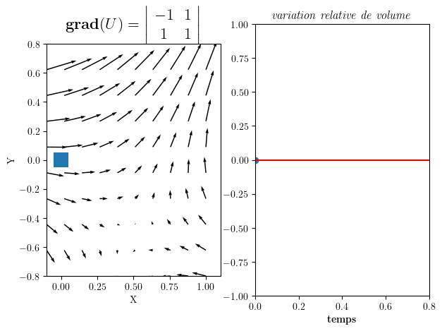
donc $\( trace(\mathbf{grad} \vec{U}) = 0\)$

U0=np.array([1.0,0.])
gradU=np.array([[-1,1.0],[1.,1.0]])
anim=part_animation(U0,gradU,FigSize=(7,5))

Gradient de U    = | -1 1 |
                   | 1 1 |
Divergence div(U)= 0.0
Rotation W_z     = 0.0
volume initiale  0.020000000000000004
Animation avec  40

plt.rc('animation', html='jshtml')
anim

Once Loop Reflect

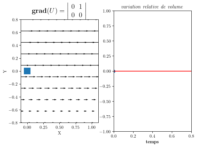
4.2.2. Cisaillement homogéne

gradU=np.array([[0,1],[0,0]])
anim=part_animation(U0,gradU,FigSize=(7,5))

Gradient de U    = | 0 1 |
                   | 0 0 |
Divergence div(U)= 0
Rotation W_z     = -0.5
volume initiale  0.020000000000000004
Animation avec  40

plt.rc('animation', html='jshtml')
anim

Once Loop Reflect

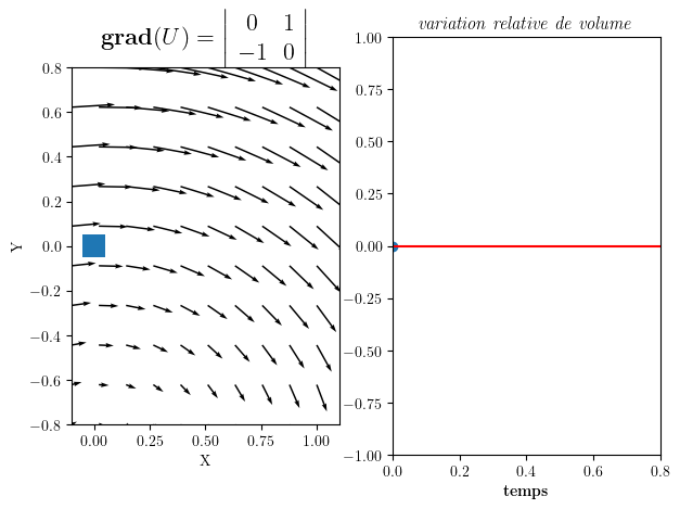
4.2.3. Rotation homogéne

gradU=np.array([[0,1],[-1,0]])
anim=part_animation(U0,gradU,FigSize=(7,5))

Gradient de U    = | 0 1 |
                   | -1 0 |
Divergence div(U)= 0
Rotation W_z     = -1.0
volume initiale  0.020000000000000004
Animation avec  40

plt.rc('animation', html='jshtml')
anim

Once Loop Reflect

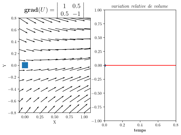
4.2.4. Déformation à volume constant

gradU=np.array([[1,0.5],[0.5,-1]])
anim=part_animation(U0,gradU,FigSize=(7,5))

Gradient de U    = | 1 0.5 |
                   | 0.5 -1 |
Divergence div(U)= 0.0
Rotation W_z     = 0.0
volume initiale  0.020000000000000004
Animation avec  40

plt.rc('animation', html='jshtml')
anim

Once Loop Reflect

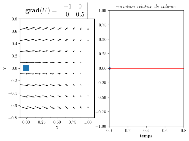
4.2.5. Compression

gradU=np.array([[-1,0.],[0.,0.5]])
anim=part_animation(U0,gradU,FigSize=(7,5))

Gradient de U    = | -1 0 |
                   | 0 0.5 |
Divergence div(U)= -0.5
Rotation W_z     = 0.0
volume initiale  0.020000000000000004
Animation avec  40

plt.rc('animation', html='jshtml')
anim

Once Loop Reflect

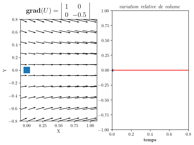
###Dilatation

gradU=np.array([[1,0.],[0.,-0.5]])
anim=part_animation(U0,gradU,FigSize=(7,5))

Gradient de U    = | 1 0 |
                   | 0 -0.5 |
Divergence div(U)= 0.5
Rotation W_z     = 0.0
volume initiale  0.020000000000000004
Animation avec  40

plt.rc('animation', html='jshtml')
anim

Once Loop Reflect

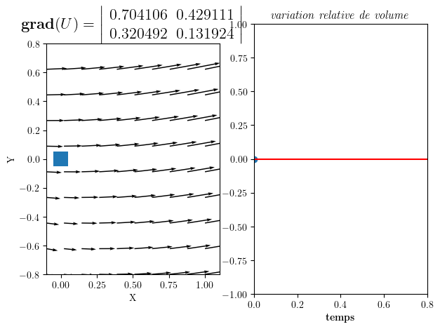
4.3. Cas Général d’un écoulement compressible

• décomposition du champ de vitesse

\[ \vec{U}(M) = \vec{U}(O) + (\nabla \vec{U})\times\vec{OM} \]

• en partie anti-symétrique (rotation) et symétrique (déformation)

\[ \vec{U}(M) = \vec{U}(O) + \vec{\Omega} \wedge \vec{OM} + D \]

gradU=np.array([np.random.rand(2),np.random.rand(2)])
anim=part_animation(U0,gradU,FigSize=(7,5))

Gradient de U    = | 0.704106 0.429111 |
                   | 0.320492 0.131924 |
Divergence div(U)= 0.8360302213464554
Rotation W_z     = -0.054309216254831705
volume initiale  0.020000000000000004
Animation avec  40

plt.rc('animation', html='jshtml')
anim

Once Loop Reflect

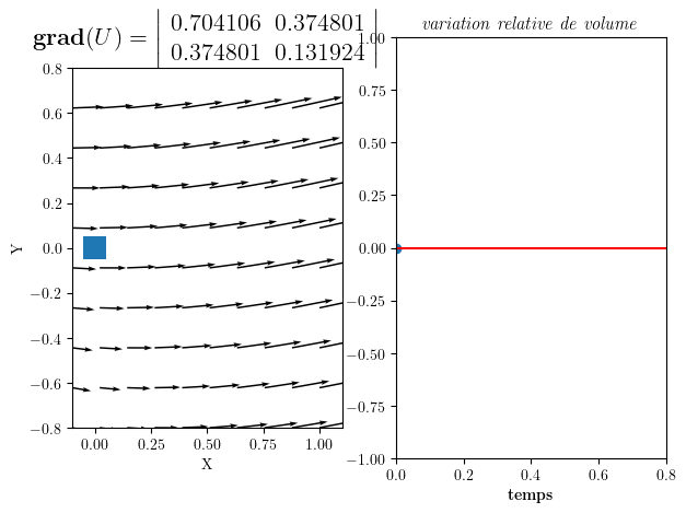
4.3.1. partie déformation (symétrique)

UZ = np.array([0.,0.])
D  = 0.5*(gradU + gradU.transpose())
anim=part_animation(U0,D,FigSize=(7,5))

Gradient de U    = | 0.704106 0.374801 |
                   | 0.374801 0.131924 |
Divergence div(U)= 0.8360302213464554
Rotation W_z     = 0.0
volume initiale  0.020000000000000004
Animation avec  40

plt.rc('animation', html='jshtml')
anim

Once Loop Reflect

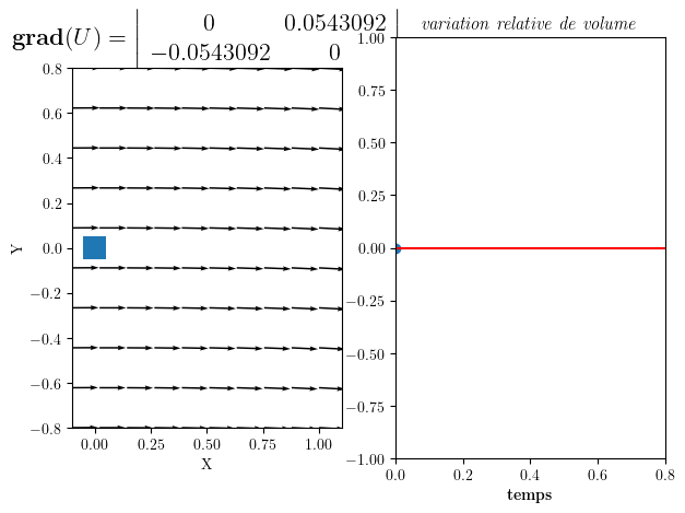
4.3.2. partie rotation(antisymétrique)

R  = 0.5*(gradU - gradU.transpose())
anim=part_animation(U0,R,FigSize=(7,5))

Gradient de U    = | 0 0.0543092 |
                   | -0.0543092 0 |
Divergence div(U)= 0.0
Rotation W_z     = -0.054309216254831705
volume initiale  0.020000000000000004
Animation avec  40

plt.rc('animation', html='jshtml')
anim

Once Loop Reflect

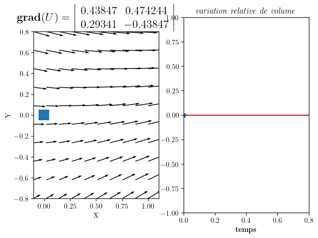
4.4. Cas Général d’un écoulement incompressible

gradU=np.array([np.random.rand(2),np.random.rand(2)])
gradU[1,1]=-gradU[0,0]
anim=part_animation(U0,gradU,FigSize=(7,5))

Gradient de U    = | 0.43847 0.474244 |
                   | 0.29341 -0.43847 |
Divergence div(U)= 0.0
Rotation W_z     = -0.09041675740406757
volume initiale  0.020000000000000004
Animation avec  40

plt.rc('animation', html='jshtml')
anim

Once Loop Reflect

4.5. FIN