3.5. Analyse aérodynamique d’une éolienne avec Xfoil#
Marc BUFFAT, département mécanique, UCB Lyon 1
%matplotlib inline
import sympy as sp
import numpy as np
import matplotlib.pyplot as plt
from validation.validation import check_function,bib_validation,exec_validation,info_etudiant
from validation.valide_markdown import test_markdown, test_code, test_algorithme
bib_validation('cours','MGC1061M')
#from Naca import Naca
3.5.1. Xfoil#
XFOIL est un programme pour la conception et l’analyse de profils isolés subsoniques développé au MIT dans les années 90 (https://web.mit.edu/drela/Public/web/xfoil/).
Il permet :
une analyse visqueuse (ou non visqueuse) d’un profil aérodynamique existant avec prise en compte de - transition forcée ou libre - séparation limitée du bord de fuite - correction de compressibilité de Karman-Tsien - nombres de Reynolds et/ou de Mach fixes ou variables
un calcul potentiel (avec une méthode de singularité des panneaux) couplé à un calcul de couche limite
Xfoil est écrit en Fortran 90 et on utilise une bibliothèque Python permettant de l’utiliser directement dans un programme Python.
3.5.1.1. documentation originale#
https://jupyterm1.mecanique.univ-lyon1.fr/cours_html/MGC1061M
from xfoil import XFoil
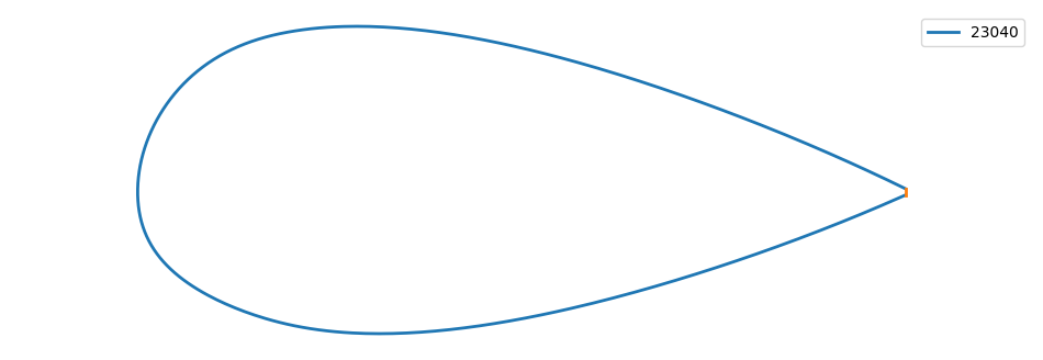
3.5.1.2. création d’une structure XFoil et définition du profil#
xf = XFoil()
naca_id = "23040"
xf.naca(naca_id)
naca = xf.airfoil
 Max thickness =     0.400103  at x =   0.303
 Max camber    =     0.018385  at x =   0.148

 Buffer airfoil set using 425 points

 Blunt trailing edge.  Gap =  0.00840

 Paneling parameters used...
   Number of panel nodes       160
   Panel bunching parameter    1.000
   TE/LE panel density ratio   0.150
   Refined-area/LE panel density ratio    0.200
   Top    side refined area x/c limits  1.000 1.000
   Bottom side refined area x/c limits  1.000 1.000
def profil_plot(Xf,Yf,Label=None):
    """trace du profil naca"""
    if Label is not None:
        plt.plot(Xf,Yf,lw=2,label=Label)
        plt.plot([Xf[-1],Xf[0]],[Yf[-1],Yf[0]],lw=2)

    else:
        plt.plot(Xf,Yf,[Xf[-1],Xf[0]],[Yf[-1],Yf[0]],lw=2)
    plt.axis('equal')
    plt.axis('off')
    return
plt.figure(figsize=(12,4))
profil_plot(naca.x,naca.y,naca_id)
plt.legend();
3.5.1.3. définition des carcatéristiques d’un profil#
étude en fonction de l’angle \(\alpha\)
on spécifie le nombre de Reynolds
\(C_L\) coefficiant de portance: projection suivant \(\vec{N}=[-\sin\alpha, \cos\alpha]\) \(\perp\) à \(\vec{U}_0\)
\(C_m\) coefficient de moment (moment pression) par rapport à un point de référence \(P=[x_{ref}=0.25, y_{ref}=0]\) , qui n’est donc pas nécessairement sur la ligne moyenne à 1/4 de corde
on calcul alors le moment en un point Q quelconque par la relation de transport
d’où la position du centre de poussée exacte / à \(P\) \(x,y\) (erreur)
3.5.1.4. calcul avec xfoil#
toutes les quantités calculées sont adimensionnalisées par la dynamique de l’écoulement amont $\(q = \frac{1}{2} \rho U_0^2 \)\(. Donc un calcul sans dimension assume que le profil est tq \)Lc=1$ (vria pour les profils NACA générés)
Portance \(Cl = L/q\)
trainée \(Cd = D/q\)
moment par rapport au 1/4 corde (xp=0.25, yp=0) \(Cm = M/q\)
calcul pour un angle alpha fixé (en degré)
cl, cd, cm, cp = xf.a(angle)
distribution de pression
xp,Pr = xf.get_cp_distribution()
nombre de Reynolds \(Re=U_0/\nu\) = 0
affichage du calcul
xf.print = True / False
xf.Re = 1.e7
#xf.Re = 0
xf.print = True
cl, cd, cm, cp = xf.a(10)
print("resultat : ",cl,cd,cm,cd)
 Calculating unit vorticity distributions ...
 Calculating wake trajectory ...
 Calculating source influence matrix ...

 Solving BL system ...

 Initializing BL ...
    side            1  ...
 MRCHUE: Inverse mode at  60     Hk =   7.727
 MRCHUE: Inverse mode at  61     Hk =   2.500
 MRCHUE: Inverse mode at  93     Hk =   2.500
 MRCHUE: Inverse mode at  94     Hk =   2.500
 MRCHUE: Inverse mode at  95     Hk =   2.500
 MRCHUE: Convergence failed at  96  side 1    Res =  0.5647E+01
 MRCHUE: Inverse mode at  97     Hk =   2.500
 MRCHUE: Convergence failed at  98  side 1    Res =  0.2763E+02
    side            2  ...
 MRCHUE: Inverse mode at  48     Hk =   2.500
 MRCHUE: Inverse mode at  63     Hk =   2.500
 MRCHUE: Convergence failed at  64  side 2    Res =  0.2442E+02
 MRCHUE: Convergence failed at  66  side 2    Res =  0.5781E-01

 MRCHDU: Convergence failed at  96  side 1    Res =  0.1845E+01
 MRCHDU: Convergence failed at  97  side 1    Res =  0.1848E+01
 MRCHDU: Convergence failed at  98  side 1    Res =  0.6353E+02
 MRCHDU: Convergence failed at  64  side 2    Res =  0.1856E+01
 MRCHDU: Convergence failed at  66  side 2    Res =  0.6215E-01
 Side 1  free  transition at x/c =  0.1861   60
 Side 2  free  transition at x/c =  0.5777   49

   1   rms: 0.9413E+00   max: 0.5458E+01   D at   66  2   RLX: 0.211
       a = 10.000      CL =  1.5533
      Cm = -0.0939     CD =  0.00231   =>   CDf =  0.00511    CDp = -0.00280

 Side 1  free  transition at x/c =  0.1864   60
 Side 2  free  transition at x/c =  0.5633   49

   2   rms: 0.6081E+00   max: 0.3344E+01   D at   66  2   RLX: 0.359
       a = 10.000      CL =  1.4300
      Cm = -0.0668     CD =  0.00442   =>   CDf =  0.00526    CDp = -0.00084

 MRCHDU: Convergence failed at  67  side 2    Res =  0.1360E+01
 Side 1  free  transition at x/c =  0.1867   59
 Side 2  free  transition at x/c =  0.5576   49

   3   rms: 0.7747E+00   max: 0.3610E+01   D at   69  2   RLX: 0.365
       a = 10.000      CL =  1.1819
      Cm = -0.0244     CD =  0.00814   =>   CDf =  0.00527    CDp =  0.00287

 MRCHDU: Convergence failed at  69  side 2    Res =  0.3555E+01
 MRCHDU: Convergence failed at  70  side 2    Res =  0.6018E+01
 MRCHDU: Convergence failed at  71  side 2    Res =  0.5236E+01
 Side 1  free  transition at x/c =  0.1869   59
 Side 2  free  transition at x/c =  0.5482   50

   4   rms: 0.3880E+00   max: 0.1903E+01   D at   90  1   RLX: 0.623
       a = 10.000      CL =  0.9261
      Cm =  0.0227     CD =  0.01527   =>   CDf =  0.00530    CDp =  0.00998

 Side 1  free  transition at x/c =  0.2001   58
 Side 2  free  transition at x/c =  0.5355   52

   5   rms: 0.9554E-01   max: 0.7377E+00   D at   86  1
       a = 10.000      CL =  0.8050
      Cm =  0.0455     CD =  0.02082   =>   CDf =  0.00487    CDp =  0.01595

 Side 1  free  transition at x/c =  0.2049   58
 Side 2  free  transition at x/c =  0.5338   51

   6   rms: 0.1301E-01   max: -.1807E+00   D at   86  1
       a = 10.000      CL =  0.8172
      Cm =  0.0442     CD =  0.02005   =>   CDf =  0.00474    CDp =  0.01531

 Side 1  free  transition at x/c =  0.2033   58
 Side 2  free  transition at x/c =  0.5342   51

   7   rms: 0.1730E-01   max: 0.1403E+00   D at   84  1
       a = 10.000      CL =  0.8035
      Cm =  0.0455     CD =  0.02081   =>   CDf =  0.00476    CDp =  0.01605

 Side 1  free  transition at x/c =  0.2034   58
 Side 2  free  transition at x/c =  0.5340   51

   8   rms: 0.6456E-02   max: -.6078E-01   D at   84  1
       a = 10.000      CL =  0.8085
      Cm =  0.0450     CD =  0.02050   =>   CDf =  0.00474    CDp =  0.01576

 Side 1  free  transition at x/c =  0.2034   58
 Side 2  free  transition at x/c =  0.5341   51

   9   rms: 0.1136E-02   max: -.1137E-01   D at   84  1
       a = 10.000      CL =  0.8094
      Cm =  0.0449     CD =  0.02046   =>   CDf =  0.00475    CDp =  0.01571

 Side 1  free  transition at x/c =  0.2034   58
 Side 2  free  transition at x/c =  0.5341   51

  10   rms: 0.7709E-04   max: -.7240E-03   D at   84  1
resultat :  0.8094477653503418 0.020458463579416275 0.04492979869246483 0.020458463579416275
       a = 10.000      CL =  0.8094
      Cm =  0.0449     CD =  0.02046   =>   CDf =  0.00475    CDp =  0.01571
      9.000   12.9121   0.020458   0.007397   0.000000  -0.007397    0.2034     #
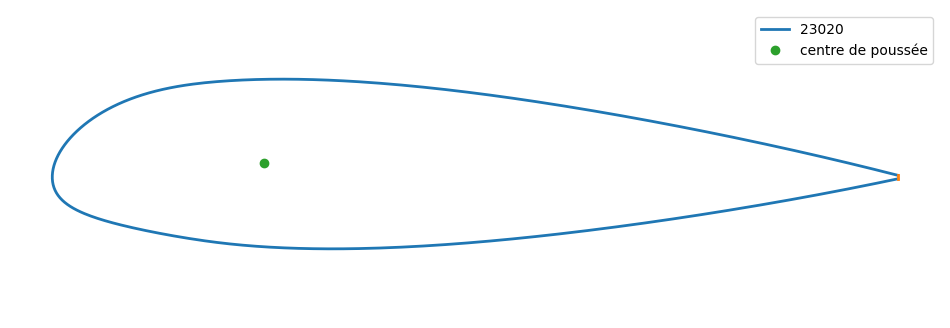
3.5.2. Etude du profil 23020#
xf = XFoil()
naca_id = "23020"
xf.naca(naca_id)
naca = xf.airfoil
X,Y = naca.x, naca.y
 Max thickness =     0.200051  at x =   0.303
 Max camber    =     0.018385  at x =   0.148

 Buffer airfoil set using 425 points

 Blunt trailing edge.  Gap =  0.00420

 Paneling parameters used...
   Number of panel nodes       160
   Panel bunching parameter    1.000
   TE/LE panel density ratio   0.150
   Refined-area/LE panel density ratio    0.200
   Top    side refined area x/c limits  1.000 1.000
   Bottom side refined area x/c limits  1.000 1.000
3.5.3. Analyse des caractéristiques aero#
# centre aerodynamique = 1/4 cordre / bord d'attaque
xp = 0.25
I=np.nonzero(np.abs(X-xp)<0.23e-2)[0]
yp = (Y[I].sum())/2.
print("centre aerodynamique :",I,xp,yp)
centre aerodynamique : [128 296] 0.25 0.01651836559176445
plt.figure(figsize=(12,4))
profil_plot(X,Y,"23020")
plt.plot([xp],[yp],'o',label="centre de poussée")
plt.legend();
3.5.3.1. portance, moment#
# analyse pour un angle fixe
Alpha=20
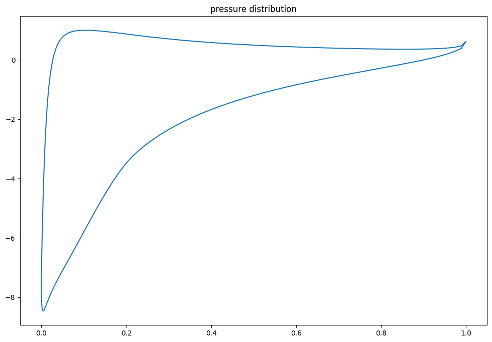
Cl, Cd, Cm, Cp = xf.a(Alpha)
print("Angle={} Lift={} Moment={} ".format(Alpha,Cl,Cm))
Xp,Pr = xf.get_cp_distribution()
plt.figure(figsize=(12,8))
plt.plot(Xp,Pr)
plt.title("pressure distribution")
 Calculating unit vorticity distributions ...
Angle=20 Lift=2.654982805252075 Moment=-0.0730389952659607
Text(0.5, 1.0, 'pressure distribution')
# centre de poussée
d = Cm/Cl
print("Position Centre de poussée:",d,xp,xp+d)
Position Centre de poussée: -0.02751015755035222 0.25 0.22248984244964778
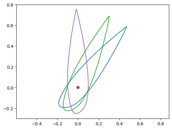
3.5.3.2. translation du profil / centre aero#
# translation du profil / au centre de poussé
print("centre de poussée :",xp,yp)
Xt = X - xp
Yt = Y - yp
centre de poussée : 0.25 0.01651836559176445
def trace_profil_rotation(X,Y,theta):
    """trace du profil avec une rotation de theta en degre"""
    ca = np.cos(theta*np.pi/180)
    sa = np.sin(theta*np.pi/180)
    X1 =  ca*X + sa*Y
    Y1 = -sa*X + ca*Y
    plt.plot(X1,Y1)
    plt.plot([0],[0],'o')
    plt.axis('equal')
    return
trace_profil_rotation(Yt,Xt,40)
trace_profil_rotation(Yt,Xt,25)
trace_profil_rotation(Yt,Xt,0)
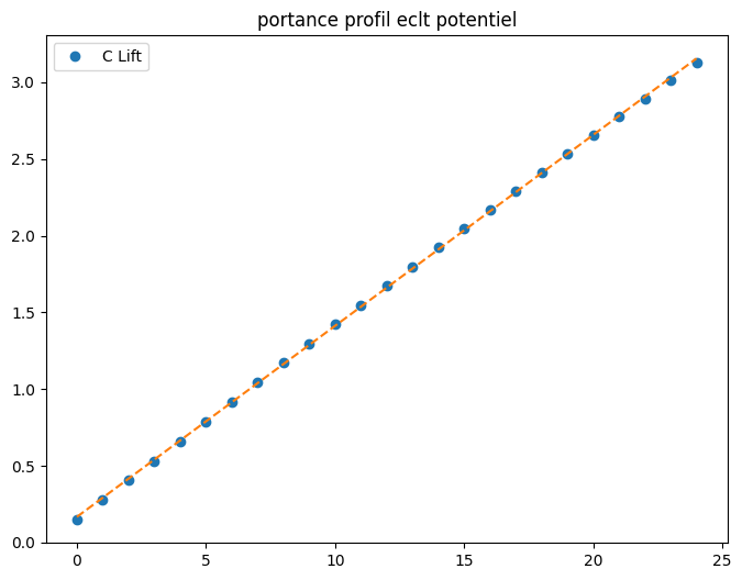
# calcul portance fluide parfait pour # angles
alpha, cl, cd, cm, cp  = xf.aseq(0,25,1)
from scipy import stats
a1,a0,r_v,r_p,err = stats.linregress(alpha,cl)
print("loi portance CL= {:.2f}*alpha + {:.2f}".format(a1,a0))
loi portance CL= 0.12*alpha + 0.17
plt.figure(figsize=(8,6))
plt.plot(alpha,cl,'o',label="C Lift")
plt.plot(alpha,a1*alpha+a0,'--')
plt.title("portance profil eclt potentiel")
plt.legend();
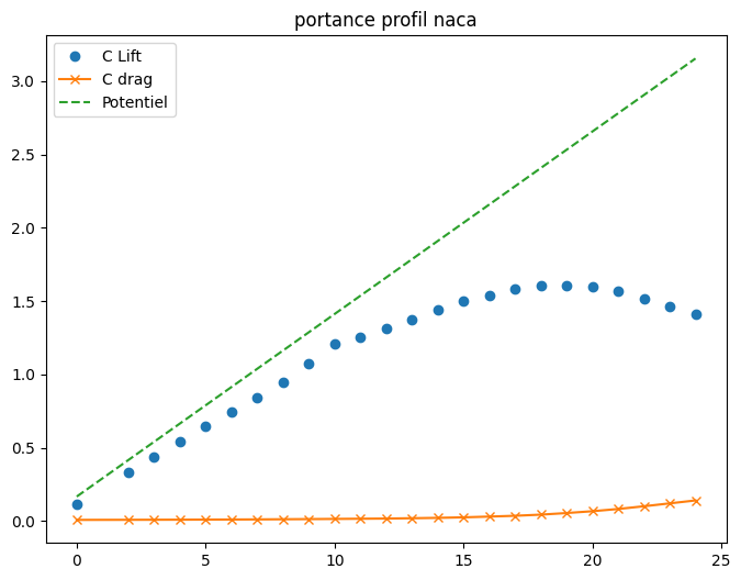
# prise en compte de la viscosite
xf.Re = 1000000
alpha, cl, cd, cm, cp  = xf.aseq(0,25,1)
 Calculating wake trajectory ...
 Calculating source influence matrix ...
 Solving BL system ...

 Initializing BL ...
    side            1  ...
 MRCHUE: Inverse mode at  50     Hk =   4.957
 MRCHUE: Inverse mode at  51     Hk =   4.580
 MRCHUE: Inverse mode at  52     Hk =   2.500
 MRCHUE: Inverse mode at  81     Hk =   2.500
 MRCHUE: Inverse mode at  82     Hk =   2.500
    side            2  ...
 MRCHUE: Inverse mode at  56     Hk =   4.936
 MRCHUE: Inverse mode at  57     Hk =   6.218
 MRCHUE: Inverse mode at  58     Hk =   6.288
 MRCHUE: Inverse mode at  59     Hk =   2.500
 MRCHUE: Inverse mode at  80     Hk =   2.500

 Side 1  free  transition at x/c =  0.3697   51
 Side 2  free  transition at x/c =  0.5556   58

   1   rms: 0.2388E+00   max: 0.1249E+01   D at   83  2   RLX: 0.648
       a =  0.000      CL =  0.1057
      Cm = -0.0030     CD =  0.00690   =>   CDf =  0.00617    CDp =  0.00072

 Side 1  free  transition at x/c =  0.3886   52
 Side 2  free  transition at x/c =  0.5778   59

   2   rms: 0.6967E-01   max: -.3233E+00   T at   59  2
       a =  0.000      CL =  0.1097
      Cm = -0.0038     CD =  0.00818   =>   CDf =  0.00605    CDp =  0.00213

 Side 1  free  transition at x/c =  0.4313   54
 Side 2  free  transition at x/c =  0.6190   61

   3   rms: 0.2660E-01   max: -.4114E+00   C at   54  1
       a =  0.000      CL =  0.1172
      Cm = -0.0054     CD =  0.00781   =>   CDf =  0.00560    CDp =  0.00221

 Side 1  free  transition at x/c =  0.4207   54
 Side 2  free  transition at x/c =  0.6193   61

   4   rms: 0.2943E-02   max: 0.4226E-01   C at   61  2
       a =  0.000      CL =  0.1160
      Cm = -0.0052     CD =  0.00790   =>   CDf =  0.00556    CDp =  0.00234

 Side 1  free  transition at x/c =  0.4191   54
 Side 2  free  transition at x/c =  0.6178   61

   5   rms: 0.4285E-04   max: -.7058E-03   C at   61  2
       a =  0.000      CL =  0.1160
      Cm = -0.0052     CD =  0.00790   =>   CDf =  0.00557    CDp =  0.00233
      9.000    3.3757   0.007902   0.000000   0.000000   0.000000    0.4191     #
 Calculating wake trajectory ...
 Calculating source influence matrix ...

 Solving BL system ...

 Side 1  free  transition at x/c =  0.4191   54
 Side 2  free  transition at x/c =  0.6178   61

   1   rms: 0.1675E+00   max: 0.1275E+01   C at   54  1   RLX: 0.492
       a =  1.000      CL =  0.1686
      Cm = -0.0046     CD =  0.00808   =>   CDf =  0.00557    CDp =  0.00251

 Side 1  free  transition at x/c =  0.3922   52
 Side 2  free  transition at x/c =  0.6343   62

   2   rms: 0.7926E-01   max: -.5816E+00   C at   62  2   RLX: 0.860
       a =  1.000      CL =  0.2178
      Cm = -0.0045     CD =  0.00802   =>   CDf =  0.00565    CDp =  0.00237

 Side 1  free  transition at x/c =  0.3688   52
 Side 2  free  transition at x/c =  0.6475   62

   3   rms: 0.3439E-01   max: -.4154E+00   C at   62  2
       a =  1.000      CL =  0.2248
      Cm = -0.0043     CD =  0.00803   =>   CDf =  0.00584    CDp =  0.00220

 Side 1  free  transition at x/c =  0.3675   52
 Side 2  free  transition at x/c =  0.6870   63

   4   rms: 0.2103E-01   max: -.4007E+00   C at   63  2
       a =  1.000      CL =  0.2223
      Cm = -0.0038     CD =  0.00803   =>   CDf =  0.00562    CDp =  0.00241

 Side 1  free  transition at x/c =  0.3677   52
 Side 2  free  transition at x/c =  0.6673   62

   5   rms: 0.3904E-02   max: -.6615E-01   C at   62  2
       a =  1.000      CL =  0.2241
      Cm = -0.0042     CD =  0.00814   =>   CDf =  0.00568    CDp =  0.00246

 Side 1  free  transition at x/c =  0.3674   52
 Side 2  free  transition at x/c =  0.6676   62

   6   rms: 0.4730E-02   max: -.1063E+00   C at   62  2
       a =  1.000      CL =  0.2241
      Cm = -0.0042     CD =  0.00814   =>   CDf =  0.00569    CDp =  0.00246

 Side 1  free  transition at x/c =  0.3674   52
 Side 2  free  transition at x/c =  0.6677   62

   7   rms: 0.4695E-02   max: -.1056E+00   C at   62  2
       a =  1.000      CL =  0.2241
      Cm = -0.0042     CD =  0.00814   =>   CDf =  0.00569    CDp =  0.00246

 Side 1  free  transition at x/c =  0.3674   52
 Side 2  free  transition at x/c =  0.6677   62

   8   rms: 0.4700E-02   max: -.1057E+00   C at   62  2
       a =  1.000      CL =  0.2241
      Cm = -0.0042     CD =  0.00814   =>   CDf =  0.00569    CDp =  0.00246

 Side 1  free  transition at x/c =  0.3674   52
 Side 2  free  transition at x/c =  0.6677   62

   9   rms: 0.4699E-02   max: -.1057E+00   C at   62  2
       a =  1.000      CL =  0.2241
      Cm = -0.0042     CD =  0.00814   =>   CDf =  0.00569    CDp =  0.00246

 Side 1  free  transition at x/c =  0.3674   52
 Side 2  free  transition at x/c =  0.6677   62

  10   rms: 0.4699E-02   max: -.1057E+00   C at   62  2
       a =  1.000      CL =  0.2241
      Cm = -0.0042     CD =  0.00814   =>   CDf =  0.00569    CDp =  0.00246

 Side 1  free  transition at x/c =  0.3674   52
 Side 2  free  transition at x/c =  0.6677   62

  11   rms: 0.4699E-02   max: -.1057E+00   C at   62  2
       a =  1.000      CL =  0.2241
      Cm = -0.0042     CD =  0.00814   =>   CDf =  0.00569    CDp =  0.00246

 Side 1  free  transition at x/c =  0.3674   52
 Side 2  free  transition at x/c =  0.6677   62

  12   rms: 0.4699E-02   max: -.1057E+00   C at   62  2
       a =  1.000      CL =  0.2241
      Cm = -0.0042     CD =  0.00814   =>   CDf =  0.00569    CDp =  0.00246

 Side 1  free  transition at x/c =  0.3674   52
 Side 2  free  transition at x/c =  0.6677   62

  13   rms: 0.4699E-02   max: -.1057E+00   C at   62  2
       a =  1.000      CL =  0.2241
      Cm = -0.0042     CD =  0.00814   =>   CDf =  0.00569    CDp =  0.00246

 Side 1  free  transition at x/c =  0.3674   52
 Side 2  free  transition at x/c =  0.6677   62

  14   rms: 0.4699E-02   max: -.1057E+00   C at   62  2
       a =  1.000      CL =  0.2241
      Cm = -0.0042     CD =  0.00814   =>   CDf =  0.00569    CDp =  0.00246

 Side 1  free  transition at x/c =  0.3674   52
 Side 2  free  transition at x/c =  0.6677   62

  15   rms: 0.4699E-02   max: -.1057E+00   C at   62  2
       a =  1.000      CL =  0.2241
      Cm = -0.0042     CD =  0.00814   =>   CDf =  0.00569    CDp =  0.00246

 Side 1  free  transition at x/c =  0.3674   52
 Side 2  free  transition at x/c =  0.6677   62

  16   rms: 0.4699E-02   max: -.1057E+00   C at   62  2
       a =  1.000      CL =  0.2241
      Cm = -0.0042     CD =  0.00814   =>   CDf =  0.00569    CDp =  0.00246

 Side 1  free  transition at x/c =  0.3674   52
 Side 2  free  transition at x/c =  0.6677   62

  17   rms: 0.4699E-02   max: -.1057E+00   C at   62  2
       a =  1.000      CL =  0.2241
      Cm = -0.0042     CD =  0.00814   =>   CDf =  0.00569    CDp =  0.00246

 Side 1  free  transition at x/c =  0.3674   52
 Side 2  free  transition at x/c =  0.6677   62

  18   rms: 0.4699E-02   max: -.1057E+00   C at   62  2
       a =  1.000      CL =  0.2241
      Cm = -0.0042     CD =  0.00814   =>   CDf =  0.00569    CDp =  0.00246

 Side 1  free  transition at x/c =  0.3674   52
 Side 2  free  transition at x/c =  0.6677   62

  19   rms: 0.4699E-02   max: -.1057E+00   C at   62  2
       a =  1.000      CL =  0.2241
      Cm = -0.0042     CD =  0.00814   =>   CDf =  0.00569    CDp =  0.00246

 Side 1  free  transition at x/c =  0.3674   52
 Side 2  free  transition at x/c =  0.6677   62

  20   rms: 0.4699E-02   max: -.1057E+00   C at   62  2
       a =  1.000      CL =  0.2241
      Cm = -0.0042     CD =  0.00814   =>   CDf =  0.00569    CDp =  0.00246

 Side 1  free  transition at x/c =  0.3674   52
 Side 2  free  transition at x/c =  0.6677   62

  21   rms: 0.4699E-02   max: -.1057E+00   C at   62  2
       a =  1.000      CL =  0.2241
      Cm = -0.0042     CD =  0.00814   =>   CDf =  0.00569    CDp =  0.00246

 Side 1  free  transition at x/c =  0.3674   52
 Side 2  free  transition at x/c =  0.6677   62

  22   rms: 0.4699E-02   max: -.1057E+00   C at   62  2
       a =  1.000      CL =  0.2241
      Cm = -0.0042     CD =  0.00814   =>   CDf =  0.00569    CDp =  0.00246

 Side 1  free  transition at x/c =  0.3674   52
 Side 2  free  transition at x/c =  0.6677   62

  23   rms: 0.4699E-02   max: -.1057E+00   C at   62  2
       a =  1.000      CL =  0.2241
      Cm = -0.0042     CD =  0.00814   =>   CDf =  0.00569    CDp =  0.00246

 Side 1  free  transition at x/c =  0.3674   52
 Side 2  free  transition at x/c =  0.6677   62

  24   rms: 0.4699E-02   max: -.1057E+00   C at   62  2
       a =  1.000      CL =  0.2241
      Cm = -0.0042     CD =  0.00814   =>   CDf =  0.00569    CDp =  0.00246

 Side 1  free  transition at x/c =  0.3674   52
 Side 2  free  transition at x/c =  0.6677   62

  25   rms: 0.4699E-02   max: -.1057E+00   C at   62  2
       a =  1.000      CL =  0.2241
      Cm = -0.0042     CD =  0.00814   =>   CDf =  0.00569    CDp =  0.00246
 VISCAL:  Convergence failed
      9.000    3.4125   0.008142   0.000000   0.000000   0.000000    0.3674     #
 Calculating wake trajectory ...
 Calculating source influence matrix ...

 Solving BL system ...

 Side 1  free  transition at x/c =  0.3674   52
 Side 2  free  transition at x/c =  0.6677   62

   1   rms: 0.1521E+00   max: 0.1226E+01   C at   52  1   RLX: 0.865
       a =  2.000      CL =  0.3219
      Cm = -0.0041     CD =  0.00849   =>   CDf =  0.00560    CDp =  0.00289

 Side 1  free  transition at x/c =  0.3248   52
 Side 2  free  transition at x/c =  0.7094   62

   2   rms: 0.2288E-01   max: -.1722E+00   D at   52  1
       a =  2.000      CL =  0.3318
      Cm = -0.0031     CD =  0.00849   =>   CDf =  0.00580    CDp =  0.00269

 Side 1  free  transition at x/c =  0.3189   52
 Side 2  free  transition at x/c =  0.7249   63

   3   rms: 0.3063E-02   max: 0.5483E-01   C at   63  2
       a =  2.000      CL =  0.3303
      Cm = -0.0028     CD =  0.00844   =>   CDf =  0.00572    CDp =  0.00273

 Side 1  free  transition at x/c =  0.3189   52
 Side 2  free  transition at x/c =  0.7228   63

   4   rms: 0.4797E-04   max: -.1022E-02   D at   64  2
       a =  2.000      CL =  0.3303
      Cm = -0.0028     CD =  0.00845   =>   CDf =  0.00573    CDp =  0.00272
      9.000    3.5416   0.008445   0.000000   0.000000   0.000000    0.3189     #
 Calculating wake trajectory ...
 Calculating source influence matrix ...

 Solving BL system ...

 Side 1  free  transition at x/c =  0.3189   52
 Side 2  free  transition at x/c =  0.7228   63

   1   rms: 0.1647E+00   max: -.1105E+01   D at   52  1   RLX: 0.453
       a =  3.000      CL =  0.3770
      Cm = -0.0020     CD =  0.00869   =>   CDf =  0.00567    CDp =  0.00302

 Side 1  free  transition at x/c =  0.2993   52
 Side 2  free  transition at x/c =  0.7348   63

   2   rms: 0.9747E-01   max: -.5606E+00   C at   63  2   RLX: 0.892
       a =  3.000      CL =  0.4305
      Cm = -0.0019     CD =  0.00882   =>   CDf =  0.00589    CDp =  0.00293

 Side 1  free  transition at x/c =  0.2802   51
 Side 2  free  transition at x/c =  0.7888   65

   3   rms: 0.1919E-01   max: 0.2758E+00   C at   65  2
       a =  3.000      CL =  0.4361
      Cm = -0.0015     CD =  0.00887   =>   CDf =  0.00573    CDp =  0.00314

 Side 1  free  transition at x/c =  0.2791   51
 Side 2  free  transition at x/c =  0.7771   64

   4   rms: 0.1253E-02   max: -.1848E-01   C at   64  2
       a =  3.000      CL =  0.4360
      Cm = -0.0015     CD =  0.00887   =>   CDf =  0.00578    CDp =  0.00309

 Side 1  free  transition at x/c =  0.2788   51
 Side 2  free  transition at x/c =  0.7770   64

   5   rms: 0.1343E-04   max: -.2283E-03   D at   51  1
       a =  3.000      CL =  0.4360
      Cm = -0.0015     CD =  0.00887   =>   CDf =  0.00578    CDp =  0.00309
      9.000    3.8538   0.008874   0.000000   0.000000   0.000000    0.2788     #
 Calculating wake trajectory ...
 Calculating source influence matrix ...

 Solving BL system ...

 Side 1  free  transition at x/c =  0.2788   51
 Side 2  free  transition at x/c =  0.7770   64

   1   rms: 0.1501E+00   max: -.7770E+00   D at   51  1   RLX: 0.643
       a =  4.000      CL =  0.5033
      Cm = -0.0006     CD =  0.00936   =>   CDf =  0.00571    CDp =  0.00365

 Side 1  free  transition at x/c =  0.2588   50
 Side 2  free  transition at x/c =  0.8085   65

   2   rms: 0.5699E-01   max: -.3897E+00   C at   65  2
       a =  4.000      CL =  0.5421
      Cm = -0.0001     CD =  0.00922   =>   CDf =  0.00573    CDp =  0.00349

 Side 1  free  transition at x/c =  0.2531   51
 Side 2  free  transition at x/c =  0.8217   64

   3   rms: 0.9260E-02   max: -.1665E+00   C at   64  2
       a =  4.000      CL =  0.5424
      Cm = -0.0003     CD =  0.00932   =>   CDf =  0.00581    CDp =  0.00350

 Side 1  free  transition at x/c =  0.2527   51
 Side 2  free  transition at x/c =  0.8301   65

   4   rms: 0.1728E-02   max: -.2545E-01   D at   66  2
       a =  4.000      CL =  0.5418
      Cm = -0.0001     CD =  0.00929   =>   CDf =  0.00574    CDp =  0.00355

 Side 1  free  transition at x/c =  0.2527   51
 Side 2  free  transition at x/c =  0.8289   65

   5   rms: 0.3507E-04   max: -.6866E-03   D at   66  2
       a =  4.000      CL =  0.5418
      Cm = -0.0001     CD =  0.00929   =>   CDf =  0.00574    CDp =  0.00354
      9.000    4.2456   0.009288   0.001261   0.001380   0.000119    0.2527     #
 Calculating wake trajectory ...
 Calculating source influence matrix ...

 Solving BL system ...

 Side 1  free  transition at x/c =  0.2527   51
 Side 2  free  transition at x/c =  0.8288   65

   1   rms: 0.1504E+00   max: -.8384E+00   C at   65  2   RLX: 0.596
       a =  5.000      CL =  0.6034
      Cm =  0.0010     CD =  0.00957   =>   CDf =  0.00566    CDp =  0.00391

 Side 1  free  transition at x/c =  0.2417   51
 Side 2  free  transition at x/c =  0.8443   64

   2   rms: 0.6003E-01   max: -.3165E+00   T at   64  2
       a =  5.000      CL =  0.6487
      Cm =  0.0008     CD =  0.00985   =>   CDf =  0.00585    CDp =  0.00400

 Side 1  free  transition at x/c =  0.2338   51
 Side 2  free  transition at x/c =  0.8781   66

   3   rms: 0.8928E-02   max: 0.1482E+00   C at   66  2
       a =  5.000      CL =  0.6457
      Cm =  0.0015     CD =  0.00981   =>   CDf =  0.00570    CDp =  0.00411

 Side 1  free  transition at x/c =  0.2342   51
 Side 2  free  transition at x/c =  0.8770   66

   4   rms: 0.5619E-03   max: 0.1010E-01   C at   66  2
       a =  5.000      CL =  0.6457
      Cm =  0.0015     CD =  0.00982   =>   CDf =  0.00570    CDp =  0.00412

 Side 1  free  transition at x/c =  0.2342   51
 Side 2  free  transition at x/c =  0.8766   66

   5   rms: 0.2095E-05   max: -.3138E-04   C at   66  2
       a =  5.000      CL =  0.6457
      Cm =  0.0015     CD =  0.00982   =>   CDf =  0.00570    CDp =  0.00411
      9.000    4.6032   0.009815   0.001287   0.001463   0.000176    0.2342     #
 Calculating wake trajectory ...
 Calculating source influence matrix ...

 Solving BL system ...

 Side 1  free  transition at x/c =  0.2342   51
 Side 2  free  transition at x/c =  0.8766   66

   1   rms: 0.1439E+00   max: -.6258E+00   D at   51  1   RLX: 0.799
       a =  6.000      CL =  0.7263
      Cm =  0.0032     CD =  0.01037   =>   CDf =  0.00561    CDp =  0.00476

 Side 1  free  transition at x/c =  0.2237   51
 Side 2  free  transition at x/c =  0.9039   66

   2   rms: 0.3326E-01   max: -.2440E+00   D at   51  1
       a =  6.000      CL =  0.7488
      Cm =  0.0033     CD =  0.01035   =>   CDf =  0.00557    CDp =  0.00477

 Side 1  free  transition at x/c =  0.2210   52
 Side 2  free  transition at x/c =  0.9197   66

   3   rms: 0.8447E-02   max: 0.1489E+00   C at   66  2
       a =  6.000      CL =  0.7468
      Cm =  0.0037     CD =  0.01042   =>   CDf =  0.00564    CDp =  0.00479

 Side 1  free  transition at x/c =  0.2206   52
 Side 2  free  transition at x/c =  0.9183   66

   4   rms: 0.6085E-03   max: -.8757E-02   D at   68  2
       a =  6.000      CL =  0.7469
      Cm =  0.0037     CD =  0.01043   =>   CDf =  0.00565    CDp =  0.00478

 Side 1  free  transition at x/c =  0.2206   52
 Side 2  free  transition at x/c =  0.9179   66

   5   rms: 0.3810E-05   max: -.5509E-04   C at   66  2
       a =  6.000      CL =  0.7469
      Cm =  0.0037     CD =  0.01043   =>   CDf =  0.00565    CDp =  0.00478
      9.000    4.8288   0.010426   0.001329   0.001557   0.000228    0.2206     #
 Calculating wake trajectory ...
 Calculating source influence matrix ...

 Solving BL system ...

 Side 1  free  transition at x/c =  0.2206   52
 Side 2  free  transition at x/c =  0.9179   66

   1   rms: 0.1374E+00   max: 0.4199E+00   D at   66  2
       a =  7.000      CL =  0.8450
      Cm =  0.0063     CD =  0.01113   =>   CDf =  0.00556    CDp =  0.00557

 Side 1  free  transition at x/c =  0.2097   52
 Side 2  free  transition at x/c =  0.9480   67

   2   rms: 0.2018E-01   max: -.1895E+00   D at   52  1
       a =  7.000      CL =  0.8442
      Cm =  0.0065     CD =  0.01115   =>   CDf =  0.00563    CDp =  0.00552

 Side 1  free  transition at x/c =  0.2094   52
 Side 2  free  transition at x/c =  0.9520   67

   3   rms: 0.1769E-02   max: 0.1529E-01   C at   52  1
       a =  7.000      CL =  0.8432
      Cm =  0.0067     CD =  0.01118   =>   CDf =  0.00562    CDp =  0.00556

 Side 1  free  transition at x/c =  0.2092   52
 Side 2  free  transition at x/c =  0.9527   67

   4   rms: 0.2416E-04   max: -.3541E-03   D at   67  2
       a =  7.000      CL =  0.8432
      Cm =  0.0067     CD =  0.01118   =>   CDf =  0.00562    CDp =  0.00556
      9.000    5.1188   0.011182   0.001377   0.001653   0.000275    0.2092     #
 Calculating wake trajectory ...
 Calculating source influence matrix ...

 Solving BL system ...

 Side 1  free  transition at x/c =  0.2092   52
 Side 2  free  transition at x/c =  0.9527   67

   1   rms: 0.1332E+00   max: -.5285E+00   T at   67  2   RLX: 0.946
       a =  8.000      CL =  0.9322
      Cm =  0.0100     CD =  0.01185   =>   CDf =  0.00553    CDp =  0.00631
 Side 1  free  transition at x/c =  0.1989   53
 Side 2  free  transition at x/c =  0.9776   68

   2   rms: 0.2039E-01   max: 0.2371E+00   D at   68  2
       a =  8.000      CL =  0.9452
      Cm =  0.0078     CD =  0.01230   =>   CDf =  0.00567    CDp =  0.00663

 Side 1  free  transition at x/c =  0.1972   52
 Side 2  free  transition at x/c =  0.9786   68

   3   rms: 0.7513E-02   max: -.9539E-01   D at   52  1
       a =  8.000      CL =  0.9455
      Cm =  0.0079     CD =  0.01220   =>   CDf =  0.00566    CDp =  0.00654

 Side 1  free  transition at x/c =  0.1979   52
 Side 2  free  transition at x/c =  0.9783   68

   4   rms: 0.1868E-03   max: -.2340E-02   D at   68  2
       a =  8.000      CL =  0.9457
      Cm =  0.0079     CD =  0.01220   =>   CDf =  0.00566    CDp =  0.00654

 Side 1  free  transition at x/c =  0.1979   52
 Side 2  free  transition at x/c =  0.9783   68
   5   rms: 0.3976E-06   max: -.4245E-05   D at   68  2
       a =  8.000      CL =  0.9457
      Cm =  0.0079     CD =  0.01220   =>   CDf =  0.00566    CDp =  0.00654
      9.000    5.2443   0.012202   0.001433   0.001760   0.000327    0.1979     #
 Calculating wake trajectory ...
 Calculating source influence matrix ...

 Solving BL system ...

 Side 1  free  transition at x/c =  0.1979   52
 Side 2  free  transition at x/c =  0.9783   68

   1   rms: 0.1515E+00   max: 0.4306E+00   D at   69  2
       a =  9.000      CL =  1.0804
      Cm =  0.0023     CD =  0.01302   =>   CDf =  0.00547    CDp =  0.00754

 Side 1  free  transition at x/c =  0.1888   54
 Side 2  free  transition at x/c =  0.9868   66

   2   rms: 0.2270E-01   max: -.2789E+00   T at   66  2
       a =  9.000      CL =  1.0655
      Cm =  0.0050     CD =  0.01325   =>   CDf =  0.00567    CDp =  0.00758

 Side 1  free  transition at x/c =  0.1891   54
 Side 2  free  transition at x/c =  0.9972   67

   3   rms: 0.3567E-01   max: 0.7208E+00   C at   67  2
       a =  9.000      CL =  1.0780
      Cm =  0.0023     CD =  0.01324   =>   CDf =  0.00566    CDp =  0.00758

 Side 1  free  transition at x/c =  0.1887   54
 Side 2  free  transition at x/c =  0.9890   66

   4   rms: 0.1381E-01   max: -.1611E+00   T at   66  2
       a =  9.000      CL =  1.0666
      Cm =  0.0047     CD =  0.01325   =>   CDf =  0.00567    CDp =  0.00758

 Side 1  free  transition at x/c =  0.1891   54
 Side 2  free  transition at x/c =  0.9958   67

   5   rms: 0.2673E-01   max: 0.4739E+00   C at   67  2
       a =  9.000      CL =  1.0771
      Cm =  0.0025     CD =  0.01324   =>   CDf =  0.00566    CDp =  0.00758

 Side 1  free  transition at x/c =  0.1887   54
 Side 2  free  transition at x/c =  0.9893   67

   6   rms: 0.3351E-02   max: -.6850E-01   D at   67  2
       a =  9.000      CL =  1.0757
      Cm =  0.0027     CD =  0.01327   =>   CDf =  0.00567    CDp =  0.00759

 Side 1  free  transition at x/c =  0.1887   54
 Side 2  free  transition at x/c =  0.9898   67

   7   rms: 0.1995E-04   max: 0.3532E-03   T at   67  2
       a =  9.000      CL =  1.0757
      Cm =  0.0027     CD =  0.01327   =>   CDf =  0.00567    CDp =  0.00760
      9.000    5.2165   0.013266   0.001509   0.001846   0.000337    0.1887     #
 Calculating wake trajectory ...
 Calculating source influence matrix ...

 Solving BL system ...

 Side 1  free  transition at x/c =  0.1887   54
 Side 2  free  transition at x/c =  0.9898   67

   1   rms: 0.1558E+00   max: 0.2899E+00   D at   67  2   RLX: 0.952
       a = 10.000      CL =  1.2048
      Cm = -0.0039     CD =  0.01464   =>   CDf =  0.00546    CDp =  0.00918

 Side 1  free  transition at x/c =  0.1801   55
 Side 2  free  transition at x/c =  0.9946   65

   2   rms: 0.3303E-01   max: -.3208E+00   D at   55  1
       a = 10.000      CL =  1.2091
      Cm = -0.0036     CD =  0.01435   =>   CDf =  0.00564    CDp =  0.00872

 Side 1  free  transition at x/c =  0.1803   55
 Side 2  free  transition at x/c =  0.9966   65

   3   rms: 0.3214E-02   max: -.3361E-01   D at   56  1
       a = 10.000      CL =  1.2082
      Cm = -0.0035     CD =  0.01446   =>   CDf =  0.00565    CDp =  0.00882

 Side 1  free  transition at x/c =  0.1797   55
 Side 2  free  transition at x/c =  0.9968   65

   4   rms: 0.7887E-04   max: -.8520E-03   D at   56  1
       a = 10.000      CL =  1.2082
      Cm = -0.0034     CD =  0.01447   =>   CDf =  0.00565    CDp =  0.00881
      9.000    5.3377   0.014466   0.001584   0.001952   0.000368    0.1797     #
 Calculating wake trajectory ...
 Calculating source influence matrix ...

 Solving BL system ...

 Side 1  free  transition at x/c =  0.1797   55
 Side 2  free  transition at x/c =  0.9968   65

   1   rms: 0.1468E+00   max: -.2912E+00   T at   65  2
       a = 11.000      CL =  1.3353
      Cm = -0.0087     CD =  0.01568   =>   CDf =  0.00553    CDp =  0.01014

 Side 1  free  transition at x/c =  0.1709   55
 Side 2 forced transition at x/c =  1.0000   64

   2   rms: 0.8779E-01   max: -.6506E+00   D at   64  2   RLX: 0.768
       a = 11.000      CL =  1.2682
      Cm =  0.0039     CD =  0.01577   =>   CDf =  0.00567    CDp =  0.01011

 Side 1  free  transition at x/c =  0.1716   55
 Side 2 forced transition at x/c =  1.0000   64

   3   rms: 0.1250E-01   max: -.1120E+00   C at   64  2
       a = 11.000      CL =  1.2558
      Cm =  0.0064     CD =  0.01571   =>   CDf =  0.00567    CDp =  0.01004

 Side 1  free  transition at x/c =  0.1716   55
 Side 2 forced transition at x/c =  1.0000   64

   4   rms: 0.2291E-02   max: 0.2557E-01   C at   64  2
       a = 11.000      CL =  1.2569
      Cm =  0.0062     CD =  0.01571   =>   CDf =  0.00565    CDp =  0.01006

 Side 1  free  transition at x/c =  0.1716   55
 Side 2 forced transition at x/c =  1.0000   64

   5   rms: 0.8530E-04   max: 0.9124E-03   C at   64  2
       a = 11.000      CL =  1.2570
      Cm =  0.0062     CD =  0.01571   =>   CDf =  0.00565    CDp =  0.01006
      9.000    5.3469   0.015713   0.014192   0.002038  -0.012154    0.1716     #
 Calculating wake trajectory ...
 Calculating source influence matrix ...

 Solving BL system ...

 Side 1  free  transition at x/c =  0.1716   55
 Side 2 forced transition at x/c =  1.0000   64

   1   rms: 0.1216E+00   max: -.9058E+00   C at   64  2   RLX: 0.552
       a = 12.000      CL =  1.2805
      Cm =  0.0124     CD =  0.01613   =>   CDf =  0.00565    CDp =  0.01048

 Side 1  free  transition at x/c =  0.1694   55
 Side 2 forced transition at x/c =  1.0000   64

   2   rms: 0.5485E-01   max: 0.9315E-01   D at   69  2
       a = 12.000      CL =  1.3153
      Cm =  0.0140     CD =  0.01688   =>   CDf =  0.00545    CDp =  0.01142

 Side 1  free  transition at x/c =  0.1656   56
 Side 2 forced transition at x/c =  1.0000   63

   3   rms: 0.4157E-02   max: -.3642E-01   D at    3  1
       a = 12.000      CL =  1.3133
      Cm =  0.0141     CD =  0.01695   =>   CDf =  0.00556    CDp =  0.01140

 Side 1  free  transition at x/c =  0.1659   56
 Side 2 forced transition at x/c =  1.0000   63

   4   rms: 0.2644E-03   max: -.2453E-02   D at    4  1
       a = 12.000      CL =  1.3133
      Cm =  0.0141     CD =  0.01695   =>   CDf =  0.00555    CDp =  0.01140

 Side 1  free  transition at x/c =  0.1659   56
 Side 2 forced transition at x/c =  1.0000   63

   5   rms: 0.5679E-06   max: -.5546E-05   C at   63  2
       a = 12.000      CL =  1.3133
      Cm =  0.0141     CD =  0.01695   =>   CDf =  0.00555    CDp =  0.01140
      9.000    5.3325   0.016952   0.014237   0.002077  -0.012161    0.1659     #
 Calculating wake trajectory ...
 Calculating source influence matrix ...

 Solving BL system ...

 Side 1  free  transition at x/c =  0.1659   56
 Side 2 forced transition at x/c =  1.0000   63

   1   rms: 0.1224E+00   max: -.6379E+00   C at   63  2   RLX: 0.784
       a = 13.000      CL =  1.3654
      Cm =  0.0182     CD =  0.01833   =>   CDf =  0.00540    CDp =  0.01293

 Side 1  free  transition at x/c =  0.1602   57
 Side 2 forced transition at x/c =  1.0000   62

   2   rms: 0.3564E-01   max: 0.1862E+00   D at   93  1
       a = 13.000      CL =  1.3660
      Cm =  0.0201     CD =  0.01974   =>   CDf =  0.00555    CDp =  0.01419

 Side 1  free  transition at x/c =  0.1576   56
 Side 2 forced transition at x/c =  1.0000   62

   3   rms: 0.1911E-01   max: -.1942E+00   D at   56  1
       a = 13.000      CL =  1.3752
      Cm =  0.0191     CD =  0.01919   =>   CDf =  0.00550    CDp =  0.01370

 Side 1  free  transition at x/c =  0.1587   56
 Side 2 forced transition at x/c =  1.0000   62

   4   rms: 0.1047E-02   max: 0.7546E-02   T at   56  1
       a = 13.000      CL =  1.3759
      Cm =  0.0190     CD =  0.01920   =>   CDf =  0.00549    CDp =  0.01370

 Side 1  free  transition at x/c =  0.1585   56
 Side 2 forced transition at x/c =  1.0000   62

   5   rms: 0.8138E-05   max: -.7775E-04   C at   62  2
       a = 13.000      CL =  1.3759
      Cm =  0.0190     CD =  0.01920   =>   CDf =  0.00550    CDp =  0.01370
      9.000    6.1693   0.019197   0.014468   0.002156  -0.012312    0.1585     #
 Calculating wake trajectory ...
 Calculating source influence matrix ...

 Solving BL system ...

 Side 1  free  transition at x/c =  0.1585   56
 Side 2 forced transition at x/c =  1.0000   62

   1   rms: 0.1217E+00   max: -.3857E+00   C at   62  2
       a = 14.000      CL =  1.4531
      Cm =  0.0215     CD =  0.02110   =>   CDf =  0.00533    CDp =  0.01576

 Side 1  free  transition at x/c =  0.1513   57
 Side 2 forced transition at x/c =  1.0000   61

   2   rms: 0.1469E-01   max: 0.1132E+00   D at   92  1
       a = 14.000      CL =  1.4424
      Cm =  0.0221     CD =  0.02177   =>   CDf =  0.00543    CDp =  0.01633

 Side 1  free  transition at x/c =  0.1517   57
 Side 2 forced transition at x/c =  1.0000   61

   3   rms: 0.1078E-02   max: 0.2143E-01   D at   91  1
       a = 14.000      CL =  1.4421
      Cm =  0.0221     CD =  0.02177   =>   CDf =  0.00540    CDp =  0.01637

 Side 1  free  transition at x/c =  0.1517   57
 Side 2 forced transition at x/c =  1.0000   61

   4   rms: 0.5376E-04   max: -.6008E-03   D at   91  1
       a = 14.000      CL =  1.4422
      Cm =  0.0221     CD =  0.02177   =>   CDf =  0.00540    CDp =  0.01637
      9.000    6.9961   0.021770   0.014537   0.002198  -0.012339    0.1517     #
 Calculating wake trajectory ...
 Calculating source influence matrix ...

 Solving BL system ...

 Side 1  free  transition at x/c =  0.1517   57
 Side 2 forced transition at x/c =  1.0000   61

   1   rms: 0.1245E+00   max: -.4280E+00   D at   57  1   RLX: 0.913
       a = 15.000      CL =  1.4942
      Cm =  0.0250     CD =  0.02502   =>   CDf =  0.00522    CDp =  0.01980

 Side 1  free  transition at x/c =  0.1458   57
 Side 2 forced transition at x/c =  1.0000   60

   2   rms: 0.2238E-01   max: -.2125E+00   D at   58  1
       a = 15.000      CL =  1.5002
      Cm =  0.0247     CD =  0.02524   =>   CDf =  0.00529    CDp =  0.01996

 Side 1  free  transition at x/c =  0.1453   57
 Side 2 forced transition at x/c =  1.0000   60

   3   rms: 0.1583E-02   max: -.1913E-01   D at   58  1
       a = 15.000      CL =  1.4995
      Cm =  0.0248     CD =  0.02529   =>   CDf =  0.00526    CDp =  0.02003

 Side 1  free  transition at x/c =  0.1450   57
 Side 2 forced transition at x/c =  1.0000   60

   4   rms: 0.6143E-04   max: 0.4872E-03   D at   89  1
       a = 15.000      CL =  1.4995
      Cm =  0.0248     CD =  0.02529   =>   CDf =  0.00526    CDp =  0.02003
      9.000    7.8912   0.025290   0.014532   0.002253  -0.012279    0.1450     #
 Calculating wake trajectory ...
 Calculating source influence matrix ...

 Solving BL system ...

 Side 1  free  transition at x/c =  0.1450   57
 Side 2 forced transition at x/c =  1.0000   60

   1   rms: 0.1197E+00   max: 0.3018E+00   D at   88  1   RLX: 0.820
       a = 16.000      CL =  1.5492
      Cm =  0.0262     CD =  0.02840   =>   CDf =  0.00507    CDp =  0.02333

 Side 1  free  transition at x/c =  0.1387   58
 Side 2 forced transition at x/c =  1.0000   59

   2   rms: 0.3498E-01   max: 0.2495E+00   D at   89  1
       a = 16.000      CL =  1.5392
      Cm =  0.0273     CD =  0.03068   =>   CDf =  0.00522    CDp =  0.02546

 Side 1  free  transition at x/c =  0.1375   57
 Side 2 forced transition at x/c =  1.0000   59

   3   rms: 0.3493E-02   max: 0.4833E-01   D at   88  1
       a = 16.000      CL =  1.5402
      Cm =  0.0272     CD =  0.03046   =>   CDf =  0.00516    CDp =  0.02530

 Side 1  free  transition at x/c =  0.1376   57
 Side 2 forced transition at x/c =  1.0000   59

   4   rms: 0.5750E-03   max: -.4572E-02   D at   88  1
       a = 16.000      CL =  1.5406
      Cm =  0.0272     CD =  0.03043   =>   CDf =  0.00516    CDp =  0.02527

 Side 1  free  transition at x/c =  0.1376   57
 Side 2 forced transition at x/c =  1.0000   59

   5   rms: 0.2245E-04   max: -.1161E-03   D at   68  2
       a = 16.000      CL =  1.5406
      Cm =  0.0272     CD =  0.03043   =>   CDf =  0.00516    CDp =  0.02527
      9.000    8.8732   0.030430   0.014363   0.002306  -0.012057    0.1376     #
 Calculating wake trajectory ...
 Calculating source influence matrix ...

 Solving BL system ...

 Side 1  free  transition at x/c =  0.1376   57
 Side 2 forced transition at x/c =  1.0000   59

   1   rms: 0.1194E+00   max: -.4784E+00   C at   57  1   RLX: 0.729
       a = 17.000      CL =  1.5880
      Cm =  0.0275     CD =  0.03327   =>   CDf =  0.00495    CDp =  0.02832

 Side 1  free  transition at x/c =  0.1331   58
 Side 2 forced transition at x/c =  1.0000   58

   2   rms: 0.3736E-01   max: 0.2068E+00   D at   88  1
       a = 17.000      CL =  1.5889
      Cm =  0.0279     CD =  0.03576   =>   CDf =  0.00481    CDp =  0.03095

 Side 1  free  transition at x/c =  0.1313   59
 Side 2 forced transition at x/c =  1.0000   57

   3   rms: 0.6422E-02   max: 0.6786E-01   D at   88  1
       a = 17.000      CL =  1.5850
      Cm =  0.0280     CD =  0.03590   =>   CDf =  0.00497    CDp =  0.03093

 Side 1  free  transition at x/c =  0.1314   59
 Side 2 forced transition at x/c =  1.0000   57

   4   rms: 0.8640E-03   max: 0.1138E-01   D at   87  1
       a = 17.000      CL =  1.5846
      Cm =  0.0281     CD =  0.03590   =>   CDf =  0.00496    CDp =  0.03095

 Side 1  free  transition at x/c =  0.1314   59
 Side 2 forced transition at x/c =  1.0000   57

   5   rms: 0.4400E-04   max: 0.2114E-03   D at   67  2
       a = 17.000      CL =  1.5845
      Cm =  0.0281     CD =  0.03590   =>   CDf =  0.00496    CDp =  0.03094
      9.000    9.6797   0.035901   0.014006   0.002316  -0.011690    0.1314     #
 Calculating wake trajectory ...
 Calculating source influence matrix ...

 Solving BL system ...

 Side 1  free  transition at x/c =  0.1314   59
 Side 2 forced transition at x/c =  1.0000   57

   1   rms: 0.1253E+00   max: 0.4850E+00   D at   86  1   RLX: 0.623
       a = 18.000      CL =  1.6010
      Cm =  0.0281     CD =  0.04104   =>   CDf =  0.00497    CDp =  0.03607

 Side 1  free  transition at x/c =  0.1273   58
 Side 2 forced transition at x/c =  1.0000   57

   2   rms: 0.4546E-01   max: 0.2610E+00   D at   86  1
       a = 18.000      CL =  1.6116
      Cm =  0.0280     CD =  0.04376   =>   CDf =  0.00488    CDp =  0.03888

 Side 1  free  transition at x/c =  0.1248   58
 Side 2 forced transition at x/c =  1.0000   57

   3   rms: 0.6209E-02   max: 0.7691E-01   D at   85  1
       a = 18.000      CL =  1.6074
      Cm =  0.0282     CD =  0.04378   =>   CDf =  0.00477    CDp =  0.03902

 Side 1  free  transition at x/c =  0.1248   58
 Side 2 forced transition at x/c =  1.0000   57

   4   rms: 0.3115E-03   max: 0.6629E-02   D at   84  1
       a = 18.000      CL =  1.6073
      Cm =  0.0283     CD =  0.04374   =>   CDf =  0.00476    CDp =  0.03898

 Side 1  free  transition at x/c =  0.1248   58
 Side 2 forced transition at x/c =  1.0000   57

   5   rms: 0.1679E-04   max: 0.1870E-03   D at   84  1
       a = 18.000      CL =  1.6073
      Cm =  0.0283     CD =  0.04374   =>   CDf =  0.00476    CDp =  0.03898
      9.000   10.5079   0.043739   0.013501   0.002332  -0.011169    0.1248     #
 Calculating wake trajectory ...
 Calculating source influence matrix ...

 Solving BL system ...

 Side 1  free  transition at x/c =  0.1248   58
 Side 2 forced transition at x/c =  1.0000   57

   1   rms: 0.1168E+00   max: 0.4583E+00   D at   83  1   RLX: 0.555
       a = 19.000      CL =  1.6219
      Cm =  0.0276     CD =  0.04877   =>   CDf =  0.00453    CDp =  0.04423

 Side 1  free  transition at x/c =  0.1205   59
 Side 2 forced transition at x/c =  1.0000   56

   2   rms: 0.6492E-01   max: 0.4123E+00   D at   84  1
       a = 19.000      CL =  1.6107
      Cm =  0.0269     CD =  0.05507   =>   CDf =  0.00469    CDp =  0.05038

 Side 1  free  transition at x/c =  0.1180   58
 Side 2 forced transition at x/c =  1.0000   56

   3   rms: 0.1026E-01   max: 0.1347E+00   D at   83  1
       a = 19.000      CL =  1.6060
      Cm =  0.0271     CD =  0.05473   =>   CDf =  0.00458    CDp =  0.05015

 Side 1  free  transition at x/c =  0.1179   58
 Side 2 forced transition at x/c =  1.0000   56

   4   rms: 0.9700E-03   max: 0.2048E-01   D at   82  1
       a = 19.000      CL =  1.6059
      Cm =  0.0272     CD =  0.05462   =>   CDf =  0.00456    CDp =  0.05007

 Side 1  free  transition at x/c =  0.1179   58
 Side 2 forced transition at x/c =  1.0000   56

   5   rms: 0.5494E-04   max: 0.2901E-03   D at   82  1
       a = 19.000      CL =  1.6059
      Cm =  0.0272     CD =  0.05463   =>   CDf =  0.00456    CDp =  0.05007
      9.000   11.3123   0.054626   0.012746   0.002335  -0.010412    0.1179     #
 Calculating wake trajectory ...
 Calculating source influence matrix ...

 Solving BL system ...

 Side 1  free  transition at x/c =  0.1179   58
 Side 2 forced transition at x/c =  1.0000   56

   1   rms: 0.1106E+00   max: 0.4353E+00   D at   81  1   RLX: 0.488
       a = 20.000      CL =  1.6179
      Cm =  0.0260     CD =  0.05957   =>   CDf =  0.00433    CDp =  0.05524

 Side 1  free  transition at x/c =  0.1148   59
 Side 2 forced transition at x/c =  1.0000   55

   2   rms: 0.6683E-01   max: 0.3963E+00   D at   82  1
       a = 20.000      CL =  1.6098
      Cm =  0.0245     CD =  0.06684   =>   CDf =  0.00444    CDp =  0.06240

 Side 1  free  transition at x/c =  0.1111   59
 Side 2 forced transition at x/c =  1.0000   55

   3   rms: 0.2112E-01   max: 0.2162E+00   D at   81  1
       a = 20.000      CL =  1.5949
      Cm =  0.0244     CD =  0.06766   =>   CDf =  0.00435    CDp =  0.06331

 Side 1  free  transition at x/c =  0.1115   59
 Side 2 forced transition at x/c =  1.0000   55

   4   rms: 0.3063E-02   max: -.3866E-01   D at   81  1
       a = 20.000      CL =  1.5967
      Cm =  0.0247     CD =  0.06692   =>   CDf =  0.00429    CDp =  0.06263
 Side 1  free  transition at x/c =  0.1115   59
 Side 2 forced transition at x/c =  1.0000   55

   5   rms: 0.2313E-03   max: -.1046E-02   D at   71  2
       a = 20.000      CL =  1.5969
      Cm =  0.0247     CD =  0.06695   =>   CDf =  0.00430    CDp =  0.06265

 Side 1  free  transition at x/c =  0.1115   59
 Side 2 forced transition at x/c =  1.0000   55

   6   rms: 0.7473E-05   max: -.4790E-04   D at   68  2
       a = 20.000      CL =  1.5970
      Cm =  0.0247     CD =  0.06695   =>   CDf =  0.00430    CDp =  0.06265
      9.000   12.0335   0.066952   0.011879   0.002309  -0.009570    0.1115     #
 Calculating wake trajectory ...
 Calculating source influence matrix ...

 Solving BL system ...

 Side 1  free  transition at x/c =  0.1115   59
 Side 2 forced transition at x/c =  1.0000   55

   1   rms: 0.1497E+00   max: 0.8567E+00   D at   79  1   RLX: 0.410
       a = 21.000      CL =  1.5786
      Cm =  0.0223     CD =  0.07557   =>   CDf =  0.00431    CDp =  0.07126

 Side 1  free  transition at x/c =  0.1090   58
 Side 2 forced transition at x/c =  1.0000   55

   2   rms: 0.6713E-01   max: 0.4466E+00   D at   79  1
       a = 21.000      CL =  1.5785
      Cm =  0.0202     CD =  0.08292   =>   CDf =  0.00420    CDp =  0.07872

 Side 1  free  transition at x/c =  0.1047   58
 Side 2 forced transition at x/c =  1.0000   55

   3   rms: 0.1759E-01   max: 0.1875E+00   D at   78  1
       a = 21.000      CL =  1.5655
      Cm =  0.0204     CD =  0.08288   =>   CDf =  0.00405    CDp =  0.07884

 Side 1  free  transition at x/c =  0.1050   58
 Side 2 forced transition at x/c =  1.0000   55

   4   rms: 0.2221E-02   max: -.2764E-01   D at   78  1
       a = 21.000      CL =  1.5669
      Cm =  0.0206     CD =  0.08224   =>   CDf =  0.00401    CDp =  0.07823

 Side 1  free  transition at x/c =  0.1050   58
 Side 2 forced transition at x/c =  1.0000   55

   5   rms: 0.1417E-03   max: -.6892E-03   D at   72  2
       a = 21.000      CL =  1.5670
      Cm =  0.0205     CD =  0.08226   =>   CDf =  0.00401    CDp =  0.07824

 Side 1  free  transition at x/c =  0.1050   58
 Side 2 forced transition at x/c =  1.0000   55

   6   rms: 0.3487E-05   max: -.2577E-04   D at   69  2
       a = 21.000      CL =  1.5670
      Cm =  0.0205     CD =  0.08226   =>   CDf =  0.00401    CDp =  0.07825
      9.000   12.7908   0.082258   0.010895   0.002282  -0.008613    0.1050     #
 Calculating wake trajectory ...
 Calculating source influence matrix ...

 Solving BL system ...

 Side 1  free  transition at x/c =  0.1050   58
 Side 2 forced transition at x/c =  1.0000   55

   1   rms: 0.1423E+00   max: 0.8649E+00   D at   76  1   RLX: 0.364
       a = 22.000      CL =  1.5490
      Cm =  0.0178     CD =  0.09084   =>   CDf =  0.00403    CDp =  0.08682

 Side 1  free  transition at x/c =  0.1024   58
 Side 2 forced transition at x/c =  1.0000   55

   2   rms: 0.9787E-01   max: 0.7084E+00   D at   76  1
       a = 22.000      CL =  1.5080
      Cm =  0.0130     CD =  0.10630   =>   CDf =  0.00371    CDp =  0.10259

 Side 1  free  transition at x/c =  0.0983   58
 Side 2 forced transition at x/c =  1.0000   54

   3   rms: 0.2024E-01   max: 0.2111E+00   D at   76  1
       a = 22.000      CL =  1.5114
      Cm =  0.0139     CD =  0.10196   =>   CDf =  0.00375    CDp =  0.09821

 Side 1  free  transition at x/c =  0.0986   58
 Side 2 forced transition at x/c =  1.0000   54

   4   rms: 0.5978E-02   max: -.5766E-01   D at   76  1
       a = 22.000      CL =  1.5158
      Cm =  0.0142     CD =  0.10073   =>   CDf =  0.00371    CDp =  0.09702

 Side 1  free  transition at x/c =  0.0983   58
 Side 2 forced transition at x/c =  1.0000   54

   5   rms: 0.5945E-03   max: -.2545E-02   D at   73  2
       a = 22.000      CL =  1.5163
      Cm =  0.0142     CD =  0.10081   =>   CDf =  0.00373    CDp =  0.09709

 Side 1  free  transition at x/c =  0.0983   58
 Side 2 forced transition at x/c =  1.0000   54

   6   rms: 0.3344E-04   max: -.1872E-03   D at   69  2
       a = 22.000      CL =  1.5163
      Cm =  0.0142     CD =  0.10083   =>   CDf =  0.00373    CDp =  0.09710
      9.000   13.6190   0.100828   0.009799   0.002234  -0.007565    0.0983     #
 Calculating wake trajectory ...
 Calculating source influence matrix ...

 Solving BL system ...

 Side 1  free  transition at x/c =  0.0983   58
 Side 2 forced transition at x/c =  1.0000   54

   1   rms: 0.1358E+00   max: 0.8756E+00   D at   74  1   RLX: 0.324
       a = 23.000      CL =  1.4996
      Cm =  0.0112     CD =  0.10923   =>   CDf =  0.00374    CDp =  0.10549

 Side 1  free  transition at x/c =  0.0958   58
 Side 2 forced transition at x/c =  1.0000   54

   2   rms: 0.8198E-01   max: 0.5788E+00   D at   74  1
       a = 23.000      CL =  1.4754
      Cm =  0.0059     CD =  0.12347   =>   CDf =  0.00367    CDp =  0.11980

 Side 1  free  transition at x/c =  0.0915   57
 Side 2 forced transition at x/c =  1.0000   54

   3   rms: 0.2669E-01   max: 0.2943E+00   D at   73  1
       a = 23.000      CL =  1.4622
      Cm =  0.0055     CD =  0.12196   =>   CDf =  0.00353    CDp =  0.11843

 Side 1  free  transition at x/c =  0.0913   57
 Side 2 forced transition at x/c =  1.0000   54

   4   rms: 0.2361E-02   max: -.1924E-01   D at   74  1
       a = 23.000      CL =  1.4623
      Cm =  0.0058     CD =  0.12063   =>   CDf =  0.00347    CDp =  0.11717

 Side 1  free  transition at x/c =  0.0912   57
 Side 2 forced transition at x/c =  1.0000   54

   5   rms: 0.1350E-03   max: 0.1471E-02   D at   72  1
       a = 23.000      CL =  1.4623
      Cm =  0.0058     CD =  0.12058   =>   CDf =  0.00347    CDp =  0.11710

 Side 1  free  transition at x/c =  0.0912   57
 Side 2 forced transition at x/c =  1.0000   54

   6   rms: 0.1228E-04   max: 0.5572E-04   D at   72  1
       a = 23.000      CL =  1.4623
      Cm =  0.0058     CD =  0.12058   =>   CDf =  0.00347    CDp =  0.11711
      9.000   14.4792   0.120580   0.008773   0.002178  -0.006595    0.0912     #
 Calculating wake trajectory ...
 Calculating source influence matrix ...

 Solving BL system ...

 Side 1  free  transition at x/c =  0.0912   57
 Side 2 forced transition at x/c =  1.0000   54

   1   rms: 0.1169E+00   max: 0.7716E+00   D at   72  1   RLX: 0.295
       a = 24.000      CL =  1.4521
      Cm =  0.0028     CD =  0.12774   =>   CDf =  0.00349    CDp =  0.12426

 Side 1  free  transition at x/c =  0.0887   57
 Side 2 forced transition at x/c =  1.0000   54

   2   rms: 0.8844E-01   max: 0.6119E+00   D at   71  1
       a = 24.000      CL =  1.4247
      Cm = -0.0047     CD =  0.14527   =>   CDf =  0.00343    CDp =  0.14184

 Side 1  free  transition at x/c =  0.0841   56
 Side 2 forced transition at x/c =  1.0000   54

   3   rms: 0.2264E-01   max: 0.2316E+00   D at   71  1
       a = 24.000      CL =  1.4168
      Cm = -0.0047     CD =  0.14137   =>   CDf =  0.00330    CDp =  0.13807

 Side 1  free  transition at x/c =  0.0837   56
 Side 2 forced transition at x/c =  1.0000   54

   4   rms: 0.8188E-02   max: 0.9530E-01   D at   70  1
       a = 24.000      CL =  1.4118
      Cm = -0.0050     CD =  0.14113   =>   CDf =  0.00325    CDp =  0.13787

 Side 1  free  transition at x/c =  0.0836   56
 Side 2 forced transition at x/c =  1.0000   54

   5   rms: 0.1530E-02   max: -.1527E-01   D at   70  1
       a = 24.000      CL =  1.4125
      Cm = -0.0048     CD =  0.14051   =>   CDf =  0.00324    CDp =  0.13727

 Side 1  free  transition at x/c =  0.0836   56
 Side 2 forced transition at x/c =  1.0000   54

   6   rms: 0.1658E-03   max: -.6061E-03   D at   70  1
       a = 24.000      CL =  1.4126
      Cm = -0.0048     CD =  0.14050   =>   CDf =  0.00325    CDp =  0.13725

 Side 1  free  transition at x/c =  0.0836   56
 Side 2 forced transition at x/c =  1.0000   54

   7   rms: 0.1594E-04   max: -.1009E-03   D at   75  2
       a = 24.000      CL =  1.4126
      Cm = -0.0048     CD =  0.14051   =>   CDf =  0.00325    CDp =  0.13727
      9.000   15.3326   0.140513   0.007845   0.002119  -0.005726    0.0836     #
# attention resultat
print(alpha)
[ 0. nan  2.  3.  4.  5.  6.  7.  8.  9. 10. 11. 12. 13. 14. 15. 16. 17.
 18. 19. 20. 21. 22. 23. 24.]
I = np.isfinite(alpha)
alpha = alpha[I]
cl = cl[I]
cd = cd[I]
cm = cm[I]
plt.figure(figsize=(8,6))
plt.plot(alpha,cl,'o',label="C Lift")
plt.plot(alpha,cd,'-x',label="C drag")
plt.plot(alpha,a1*alpha+a0,'--',label="Potentiel")
plt.title("portance profil naca")
plt.legend();
3.5.3.3. Choix du point de fonctionnement#
valeur de l’angle \(\alpha\)
plt.figure(figsize=(12,8))
plt.subplot(1,2,1)
plt.plot(cd,cl)
plt.title("polaire cl=f(cd)")
plt.subplot(1,2,2)
plt.plot(alpha,cl/cd)
plt.xlabel("$\\alpha$")
plt.title("finesse");
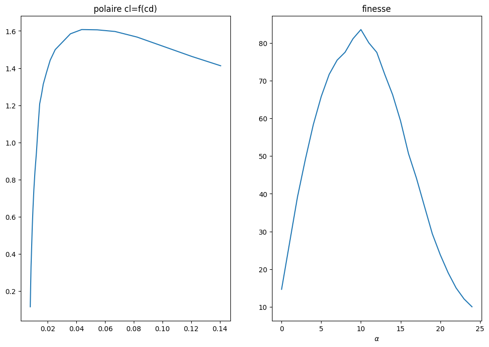
# choix du point de fonctionnement alpha
ALPHA = 12
num=np.where(alpha==ALPHA)[0][0]
print(num,ALPHA)
CD = cd[num]
CL = cl[num]
print("pt fonctionnement ALPHA={} CL={} CD={}".format(ALPHA,CL,CD))
11 12
pt fonctionnement ALPHA=12 CL=1.313344955444336 CD=0.016952097415924072
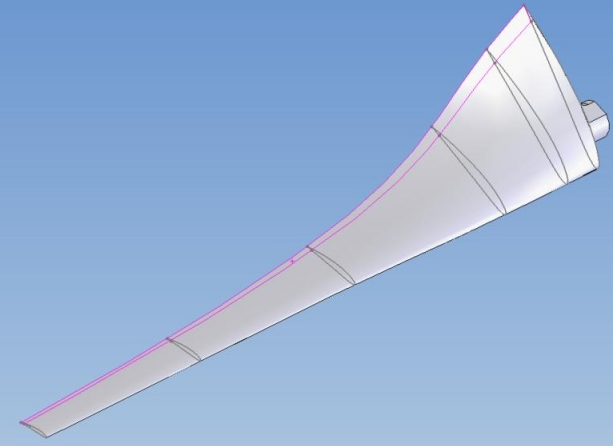
3.5.4. Etude d’une pale d’eolienne#
étude avec un profil naca 23020
3.5.4.1. caracteristique des pales#
puissance < 200kW
longueur de L= 5 a 20 m
largeur max L/10
rotation max de 400 a 100 tr/mn
rotation omega ~ 20 tr/mn
vrillage de la pale
vitesse optimale du vent V0=15 m/s
vitesse securité < 30 m/s
vitesse minimale 4 m/s
Formule de Betz pour la puissance \(P\): $\( P_{max} = 0.37 S V_0^3 \mbox{ avec } S= \pi L^2 \)$
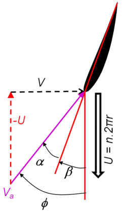
Modélisation
\(\alpha\) angle d’attaque de la pale
\(\beta\) angle de calage
\(\phi\) angle de la vitesse apparente \(V_a = V_0 - U\)
\(V_0\) vitesse vent
\(U=\omega r\) vitesse de la pale en r
direction tangentielle // à U
direction normale \(\perp\)
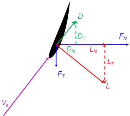
\(L\) la portance est \(\perp\) à \(V_a\)
\(L_t\) projection tangentielle de cette force engendrant une rotation de la pale
\(D\) trainée
\(D_t\) projection tangentielle de cette force opposée à la rotation de la pale
\(F_t = L_t -D_t\) résultante (utile) engendrant une puissance \(F_t \omega r\)
3.5.4.2. Calcul du calage de l’éolienne: analyse dans le plan (t,z)#
t: tangent et z: perpendiculaire au plan de l’éolienne
on veut déterminer \(\beta\) tq l’incidence \(\alpha\) reste constante alors que U varie
r, alpha, omega = sp.symbols('r alpha omega',positive=True)
U0,rho = sp.symbols('U_0 rho',positive=True)
# longueur cordre (l0 en 0 et ~0 pour r = L)
L, l0 = sp.symbols('L l_0',positive=True)
lc = l0*(L-8*r/10)
# angle de calage
U = omega*r
phi = sp.atan2(U0,U)
beta = phi - alpha
beta
angle de calage \(\beta\) tq l’angle d’incidence \(\alpha\) reste contant
# vitesse apparente
Va = sp.sqrt(U0**2+U**2)
Va
# portance et projection suivant la tangente (force utile)
Cp,Cd = sp.symbols('C_p C_d')
P  = Cp/2*rho*Va**2*lc
Pt = P*sp.cos(sp.pi/2-phi)
Pt = Pt.simplify()
display("Portance=",Pt)
# trainee
T = Cd*rho/2*Va**2*lc
Tt = -T*sp.cos(phi)
Tt = Tt.simplify()
display("Trainee ",Tt)
'Portance='
'Trainee '
# integration sur la pale pour avoir la force totale utile
FP = sp.integrate(Pt,(r,0,L)) + sp.integrate(Tt,(r,0,L))
FP = FP.simplify()
display("FP=",FP)
'FP='
# puissance totale
PP = sp.integrate(Pt*U,(r,0,L)) + sp.integrate(Tt*U,(r,0,L))
PP = PP.simplify()
display("Puissance totale=",PP)
'Puissance totale='
3.5.5. Valeurs numériques#
# Alpha angle d'incidence en degre, Omega vitesse rotation en tr/min
Alpha=ALPHA
Omega=40.
vals = {sp.pi:np.pi, l0: 1/15. , L:15. , alpha: Alpha*np.pi/180. , omega:Omega*2*np.pi/60.,
        U0:15., Cp:CL, Cd:CD, rho:1.0}
print(vals)
# formule Betz
Pmax = 0.37*(rho*sp.pi*L**2*U0**3).subs(vals)/1000
print("(Betz) Pmax={:.1f} kW".format(Pmax))
{pi: 3.141592653589793, l_0: 0.06666666666666667, L: 15.0, alpha: 0.20943951023931953, omega: 4.1887902047863905, U_0: 15.0, C_p: 1.313344955444336, C_d: 0.016952097415924072, rho: 1.0}
(Betz) Pmax=882.7 kW
display("Force totale:",FP)
print("Force portance:  {:.2f} N".format(FP.subs(vals)))
print("Puissance totale {:.2f} W".format(3*PP.subs(vals)))
'Force totale:'
Force portance:  2607.91 N
Puissance totale 247985.31 W
# estimation avec formule de Betz
Pmax = 0.37*rho*sp.pi*L**2*U0**3
print("Puissance Betz :",Pmax.subs(vals))
Puissance Betz : 882689.360888307
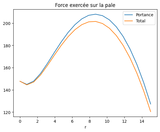
Np = 20
R  = np.linspace(0.0,float(L.subs(vals)), Np)
PT = np.array([Pt.subs(vals).subs({r:rr}) for rr in R])
FT = PT + np.array([Tt.subs(vals).subs({r:rr}) for rr in R])
plt.plot(R,PT,label="Portance")
plt.plot(R,FT,label="Total")
plt.title("Force exercée sur la pale")
plt.xlabel("r")
plt.legend();
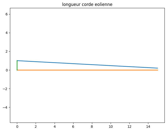
3.5.5.1. calcul du calage sur 20 secteurs#
Np = 20
R  = np.linspace(0.0,float(L.subs(vals)), Np)
Lc = np.array([lc.subs(vals).subs({r:rr}) for rr in R])
plt.figure(figsize=(8,6))
plt.plot(R,Lc,lw=2)
plt.plot(R,np.zeros(R.size),lw=2)
plt.plot([0,0],[0,Lc[0]],lw=2)
plt.axis('equal')
plt.title("longueur corde eolienne");
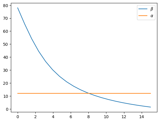
display("beta=",beta)
Beta = np.zeros(Np)
Beta[1:] = np.array([beta.subs(vals).subs({r:rr})*180./np.pi for rr in R[1:]])
Beta[0]  = 90. - Alpha
Beta
'beta='
array([78.        , 65.56730021, 54.20610468, 44.51983104, 36.59252229,
       30.21378638, 25.08876938, 20.94275254, 17.55278074, 14.7476771 ,
       12.39864428, 10.40909573,  8.7062407 ,  7.23472786,  5.95201274,
        4.8250222 ,  3.8277544 ,  2.93954306,  2.14379171,  1.42704176])
plt.plot(R,Beta,label="$\\beta$")
plt.plot(R,Alpha*np.ones(Np),label="$\\alpha$")
plt.legend()
<matplotlib.legend.Legend at 0x7fc5659b9750>
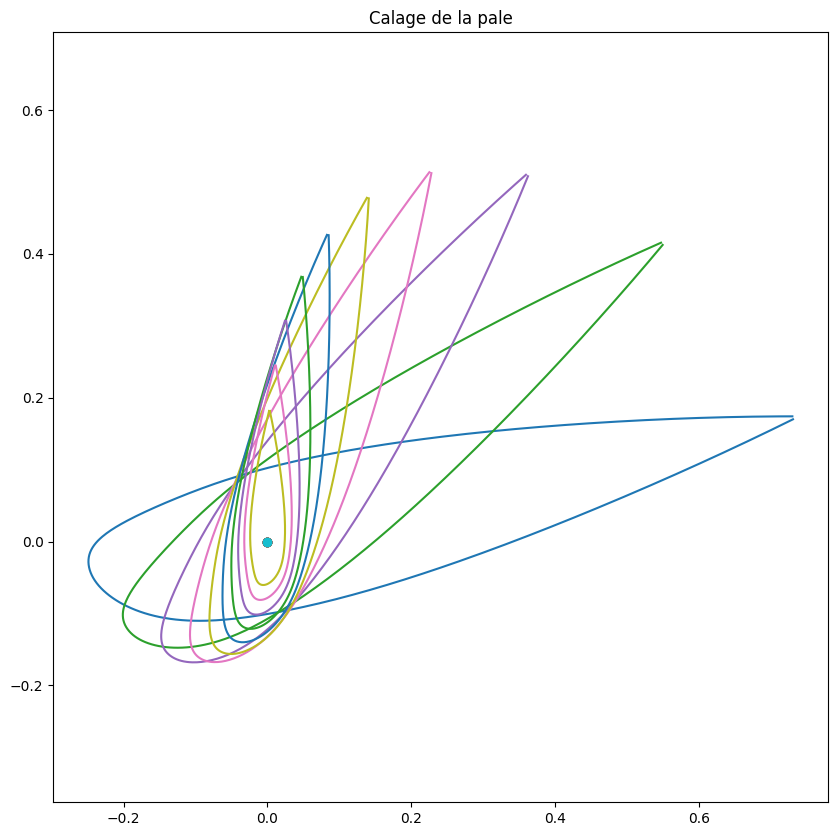
# tracer des profils
plt.figure(figsize=(10,10))
for i in range(0,Np,2):
    #print(R[i],Beta[i],Lc[i])
    trace_profil_rotation(Yt*Lc[i],Xt*Lc[i],Beta[i])
plt.title("Calage de la pale")
Text(0.5, 1.0, 'Calage de la pale')
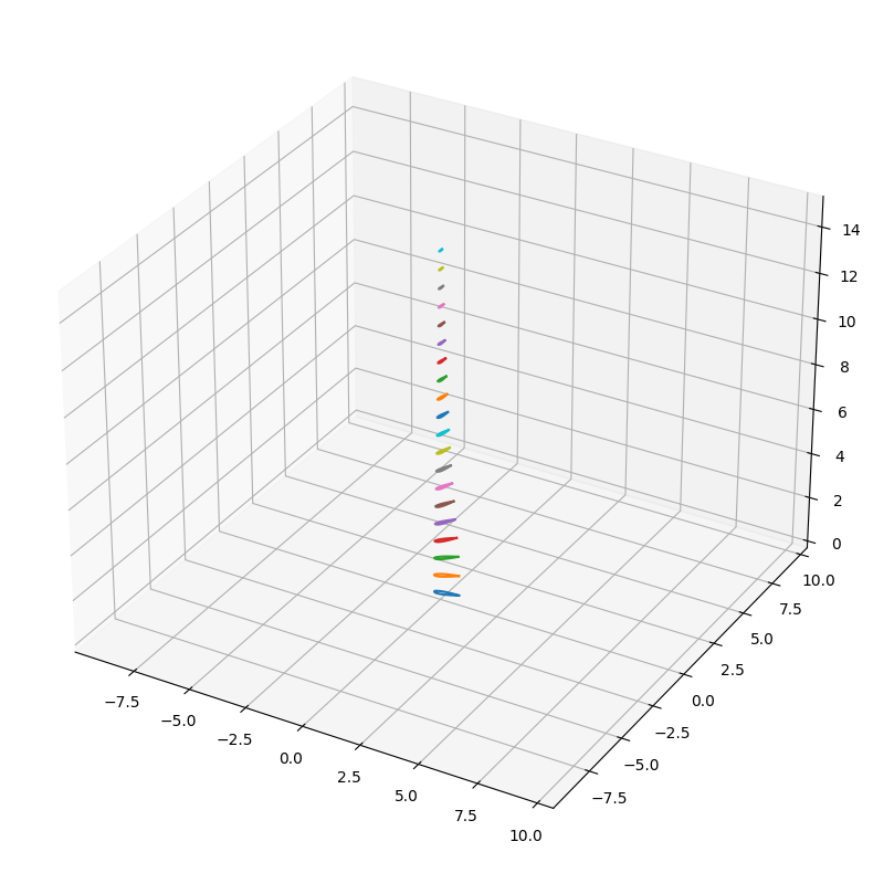
#from mpl_toolkits.mplot3d import Axes3D

def trace_profil3D(ax,X,Y,Z,theta,lw=2):
    ca = np.cos(theta*np.pi/180)
    sa = np.sin(theta*np.pi/180)
    X1 =  ca*X + sa*Y
    Y1 = -sa*X + ca*Y
    ax.plot(X1, Y1, Z)
    return
fig = plt.figure(figsize=(10,10))
ax = fig.add_subplot(111, projection='3d')
#ax  = fig.gca(projection='3d')
for i in range(0,Np,1):
    #print(i,R[i])
    trace_profil3D(ax,Yt[::4]*Lc[i],Xt[::4]*Lc[i],R[i],Beta[i])
#ax.autoscale()
#ax.set_aspect('auto')
plt.axis('equal')
plt.grid()
plt.show()