7. Time series analysis with AI/ML#
Marc Buffat dpt mécanique, UCB Lyon1
import tensorflow as tf
2026-04-09 14:16:31.640966: I external/local_xla/xla/tsl/cuda/cudart_stub.cc:32] Could not find cuda drivers on your machine, GPU will not be used.
2026-04-09 14:16:34.342688: I external/local_xla/xla/tsl/cuda/cudart_stub.cc:32] Could not find cuda drivers on your machine, GPU will not be used.
2026-04-09 14:16:35.845597: E external/local_xla/xla/stream_executor/cuda/cuda_fft.cc:467] Unable to register cuFFT factory: Attempting to register factory for plugin cuFFT when one has already been registered
WARNING: All log messages before absl::InitializeLog() is called are written to STDERR
E0000 00:00:1775736996.971129  270379 cuda_dnn.cc:8579] Unable to register cuDNN factory: Attempting to register factory for plugin cuDNN when one has already been registered
E0000 00:00:1775736997.171522  270379 cuda_blas.cc:1407] Unable to register cuBLAS factory: Attempting to register factory for plugin cuBLAS when one has already been registered
W0000 00:00:1775736999.253109  270379 computation_placer.cc:177] computation placer already registered. Please check linkage and avoid linking the same target more than once.
W0000 00:00:1775736999.253175  270379 computation_placer.cc:177] computation placer already registered. Please check linkage and avoid linking the same target more than once.
W0000 00:00:1775736999.253183  270379 computation_placer.cc:177] computation placer already registered. Please check linkage and avoid linking the same target more than once.
W0000 00:00:1775736999.253191  270379 computation_placer.cc:177] computation placer already registered. Please check linkage and avoid linking the same target more than once.
2026-04-09 14:16:39.434959: I tensorflow/core/platform/cpu_feature_guard.cc:210] This TensorFlow binary is optimized to use available CPU instructions in performance-critical operations.
To enable the following instructions: AVX2 FMA, in other operations, rebuild TensorFlow with the appropriate compiler flags.
---------------------------------------------------------------------------
KeyboardInterrupt                         Traceback (most recent call last)
Cell In[1], line 1
----> 1 import tensorflow as tf

File ~/venvs/jupyter/lib/python3.10/site-packages/tensorflow/__init__.py:49
     46 from tensorflow.python import tf2 as _tf2
     47 _tf2.enable()
---> 49 from tensorflow._api.v2 import __internal__
     50 from tensorflow._api.v2 import __operators__
     51 from tensorflow._api.v2 import audio

File ~/venvs/jupyter/lib/python3.10/site-packages/tensorflow/_api/v2/__internal__/__init__.py:11
      9 from tensorflow._api.v2.__internal__ import decorator
     10 from tensorflow._api.v2.__internal__ import dispatch
---> 11 from tensorflow._api.v2.__internal__ import distribute
     12 from tensorflow._api.v2.__internal__ import eager_context
     13 from tensorflow._api.v2.__internal__ import feature_column

File ~/venvs/jupyter/lib/python3.10/site-packages/tensorflow/_api/v2/__internal__/distribute/__init__.py:8
      3 """Public API for tf._api.v2.__internal__.distribute namespace
      4 """
      6 import sys as _sys
----> 8 from tensorflow._api.v2.__internal__.distribute import combinations
      9 from tensorflow._api.v2.__internal__.distribute import interim
     10 from tensorflow._api.v2.__internal__.distribute import multi_process_runner

File ~/venvs/jupyter/lib/python3.10/site-packages/tensorflow/_api/v2/__internal__/distribute/combinations/__init__.py:8
      3 """Public API for tf._api.v2.__internal__.distribute.combinations namespace
      4 """
      6 import sys as _sys
----> 8 from tensorflow.python.distribute.combinations import env # line: 456
      9 from tensorflow.python.distribute.combinations import generate # line: 365
     10 from tensorflow.python.distribute.combinations import in_main_process # line: 418

File ~/venvs/jupyter/lib/python3.10/site-packages/tensorflow/python/distribute/combinations.py:35
     33 from tensorflow.python.distribute import collective_all_reduce_strategy
     34 from tensorflow.python.distribute import distribute_lib
---> 35 from tensorflow.python.distribute import multi_process_runner
     36 from tensorflow.python.distribute import multi_worker_test_base
     37 from tensorflow.python.eager import context

File ~/venvs/jupyter/lib/python3.10/site-packages/tensorflow/python/distribute/multi_process_runner.py:35
     33 from tensorflow.python.compat import v2_compat
     34 from tensorflow.python.distribute import multi_worker_util
---> 35 from tensorflow.python.distribute import multi_process_lib
     36 from tensorflow.python.eager import context
     37 from tensorflow.python.framework import test_util

File ~/venvs/jupyter/lib/python3.10/site-packages/tensorflow/python/distribute/multi_process_lib.py:25
     22 from absl import app
     23 from absl import logging
---> 25 from tensorflow.python.eager import test
     28 def is_oss():
     29   """Returns whether the test is run under OSS."""

File ~/venvs/jupyter/lib/python3.10/site-packages/tensorflow/python/eager/test.py:18
     15 """Utilities for testing tfe code."""
     17 from tensorflow.python.framework import ops as _ops
---> 18 from tensorflow.python.platform import test as _test
     19 from tensorflow.python.platform.test import *  # pylint: disable=wildcard-import
     22 # TODO(akshayka): Do away with this file.

File ~/venvs/jupyter/lib/python3.10/site-packages/tensorflow/python/platform/test.py:23
     20 from unittest import mock
     22 # pylint: disable=g-bad-import-order
---> 23 from tensorflow.python.framework import test_util as _test_util
     24 from tensorflow.python.platform import googletest as _googletest
     26 # pylint: disable=unused-import

File ~/venvs/jupyter/lib/python3.10/site-packages/tensorflow/python/framework/test_util.py:91
     89 from tensorflow.python.ops.ragged import ragged_tensor_value
     90 from tensorflow.python.platform import _pywrap_stacktrace_handler
---> 91 from tensorflow.python.platform import googletest
     92 from tensorflow.python.platform import tf_logging as logging
     93 from tensorflow.python.training import server_lib

File ~/venvs/jupyter/lib/python3.10/site-packages/tensorflow/python/platform/googletest.py:30
     28 from tensorflow.python.framework import errors
     29 from tensorflow.python.lib.io import file_io
---> 30 from tensorflow.python.platform import benchmark
     31 from tensorflow.python.platform import tf_logging as logging
     32 from tensorflow.python.util import tf_decorator

File ~/venvs/jupyter/lib/python3.10/site-packages/tensorflow/python/platform/benchmark.py:30
     28 from tensorflow.core.protobuf import rewriter_config_pb2
     29 from tensorflow.core.util import test_log_pb2
---> 30 from tensorflow.python.client import timeline
     31 from tensorflow.python.framework import ops
     32 from tensorflow.python.platform import gfile

File ~/venvs/jupyter/lib/python3.10/site-packages/tensorflow/python/client/timeline.py:45
     31 class AllocationMaximum(
     32     collections.namedtuple(
     33         'AllocationMaximum', ('timestamp', 'num_bytes', 'tensors')
     34     )
     35 ):
     36   """Stores the maximum allocation for a given allocator within the timelne.
     37
     38   Parameters:
   (...)
     41     tensors: the set of tensors allocated at this time.
     42   """
---> 45 class StepStatsAnalysis(
     46     collections.namedtuple(
     47         'StepStatsAnalysis', ('chrome_trace', 'allocator_maximums')
     48     )
     49 ):
     50   """Stores the step stats analysis output.
     51
     52   Parameters:
     53     chrome_trace: A dict containing the chrome trace analysis.
     54     allocator_maximums: A dict mapping allocator names to AllocationMaximum.
     55   """
     58 class _ChromeTraceFormatter(object):

KeyboardInterrupt:
%matplotlib inline
import numpy as np
import matplotlib.pyplot as plt
# police des titres
plt.rc('font', family='serif', size='18')
from IPython.display import display,Markdown
# IA
import sklearn as sk
import tensorflow as tf
_uid_ = 12345
def serie_temp(N,a0=1.0,a1=0.5,a2 = 0.4, a3=0.1):
    # data / jours
    np.random.seed(_uid_)
    # time series
    Ts = np.array([x for x in np.arange(N)],dtype=int)
    ys = [ a0*np.sin(2*np.pi*x/180) + a1*np.cos(2*np.pi*x/15) \
         + a2*x/360  for x in range(N)] + \
           a3*np.random.normal(size=N,scale=0.2)
    return Ts,ys
7.1. Objectives#
We study a temporal system \(Y(t)\) and aim to predict the evolution of the system, i.e., the forecast of its future realizations based on its past values.
A time series \(Y(t)\) is commonly decomposed into trend, seasonality, and noise:
Trend \(T(t)\) = long-term evolution
Seasonality \(S(t)\) = periodic phenomenon
Noise \(\epsilon(t)\) = random part
7.1.1. Analysis methods#
Classical Methods (linear time series modeling):
Exponential smoothing
Regression models (linear regression, non-parametric models, etc.)
ARIMA models
An Autoregressive Integrated Moving Average (ARIMA) model is a popular statistical method for analyzing and forecasting time series data. The ARIMA model is versatile and can be used to model both stationary and non-stationary time series by incorporating differencing
SARIMA models
A Seasonal Autoregressive Integrated Moving Average (SARIMA) model is a type of statistical model used to analyze and forecast time series data that exhibits seasonality. It extends the ARIMA model by explicitly incorporating both non-seasonal and seasonal components.
7.1.2. data modelling#
Use of AI:
Random forest
Recurrent neural networks (LSTM)
7.2. Principle of the machine learning#
objective : prediction of the function \(\mathcal{F}\) s.t.
using a learning data set \(\textbf{X}_i, y_i\)
\(\rightarrow\) Minimization problem
Find the best approximation \(\mathbf{F}\) that minimizes the error \(J\) over the learning data set where \(J\) is a cost function, for example:
7.2.1. Problem#
How to define the data-set for time series
input data \(X_i\)
result data \(y_i\)
7.3. Time series data-set#
time series \(Y = Y(t)\)
N measurements at regular intervals \(\Delta t\)
data array
ys\[ys[i] = Y(i\Delta t)\]time array
ts(for the analysis)\[ts[i] = i\Delta t\]
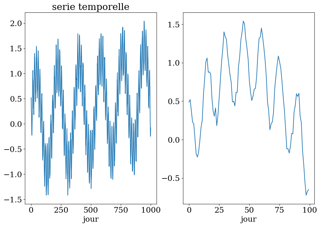
test
simple periodic series
bi-periodic series (modulation)
with long term trend
with noise
# construction serie temporelle
# cas periodique le plus simple
Ts,ys = serie_temp(1000,a0=0,a1=0.5,a2=0.0,a3 = 0.)
# cas bi-periodique
Ts,ys = serie_temp(1000,a0=1.0,a1=0.5,a2=0.0,a3=0.0)
# + tendance
Ts,ys = serie_temp(1000,a0=1.0,a1=0.5,a2=0.2,a3=0.0)
# + bruit
Ts,ys = serie_temp(1000,a0=1.0,a1=0.5,a2=0.2,a3=0.3)
plt.figure(figsize=(12,8))
plt.subplot(1,2,1)
plt.plot(Ts[:],ys)
plt.xlabel("jour")
plt.title("serie temporelle");
plt.subplot(1,2,2)
plt.plot(Ts[:100],ys[:100])
plt.xlabel("jour")
Text(0.5, 0, 'jour')
7.4. Définition of the data-set for the leraning phase#
Data Windowing:
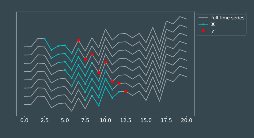
Choose a window of nav previous days to predict nap values (i.e., over the next nap days)
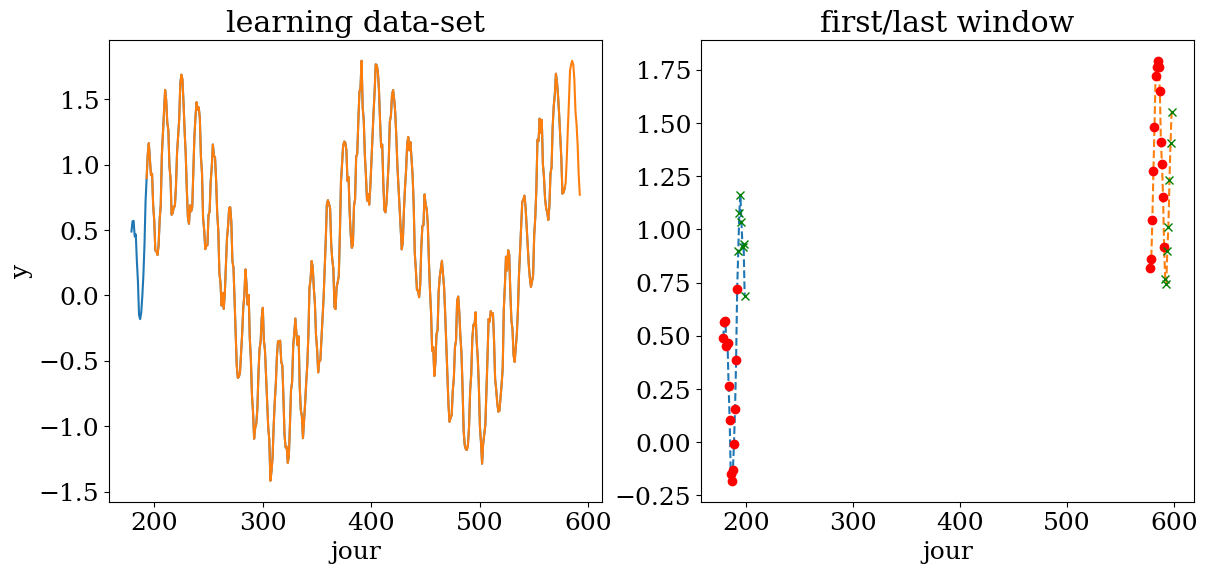
nav: size of the history window (before)nap: size of the prediction window (after)N: number of windowst0: start date for predictiont1: start date for learningt1 = t0 - (nav+nap) - N
def dataset(Ts,ys,nav,nap,N,t0):
    # choix d'une fenetre de nav jours précédents pour prédir nap valeurs (i.e. sur nap jours)
    # nav taille de la fenetre d'histoire (avant)
    # nap taille de la fenetre prediction (apres)
    # N nbre de fenetres
    # t0 date de debut prediction
    #
    t1 = t0 - N - nav -nap
    print(f"apprentissage sur {N} fenetres de {nav}-{nap} jours entre le jour {t1} et {t0}")
    #
    X  = np.zeros((N,nav))
    y  = np.zeros((N,nap))
    t  = np.zeros(N,dtype=int)
    # construction de la base de données
    for i in range(N):
        X[i,:] = ys[t1+i:t1+i+nav]
        y[i]   = ys[t1+i+nav:t1+i+nav+nap]
        t[i]   = Ts[t1+i+nav]
    return X,y,t
# N fenetres: de 14 jours -> 7 jours pour prediction à partir du jour t0
nav = 14
nap = 7
#N  = 200
#t0 = 300
N = 400
t0 = 600
X,y,t = dataset(Ts,ys,nav,nap,N,t0)
apprentissage sur 400 fenetres de 14-7 jours entre le jour 179 et 600
X.shape, y.shape, t.shape
((400, 14), (400, 7), (400,))
def plot_dataset():
    plt.figure(figsize=(14,6))
    plt.subplot(1,2,1)
    plt.plot(t-nav,X[:,0])
    plt.plot(t,y[:,0])
    plt.xlabel("jour")
    plt.ylabel("y")
    plt.title("learning data-set")
    plt.subplot(1,2,2)
    plt.plot(np.arange(t[0]-nav,t[0]+nap),ys[t[0]-nav:t[0]+nap],'--')
    plt.plot(np.arange(t[0]-nav,t[0]),X[0,:],'or')
    plt.plot(np.arange(t[0],t[0]+nap),y[0,:],'xg')
    plt.plot(np.arange(t[-1]-nav,t[-1]+nap),ys[t[-1]-nav:t[-1]+nap],'--')
    plt.plot(np.arange(t[-1]-nav,t[-1]),X[-1,:],'or')
    plt.plot(np.arange(t[-1],t[-1]+nap),y[-1,:],'xg')
    plt.xlabel("jour")
    plt.title("first/last window");
    return
plot_dataset()
7.5. Scikit Learn RandomForest#
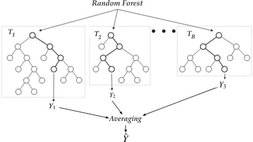
“Random Forest” of Decision Trees
Prediction of one value at a time
7.6. Neural Network: LSTM/RNN#
LSTM = Long Short-Term Memory
Recurrent neural network (RNN)
Activation function: prevents output explosion (
tanh)Numerical gradient method (learning rate \(\alpha\)):
\[ w_{k+1} = w_k - \alpha F_w \]EPOCH = number of epochs for training
The number of epochs is an hyper-parameter that defines how many times the learning algorithm goes through the entire training dataset.
7.6.1. Artificial Neuron Model#
An artificial neuron is a fundamental unit in neural networks, designed to simulate the function of a biological neuron. Here’s an overview of its key components and functionality:
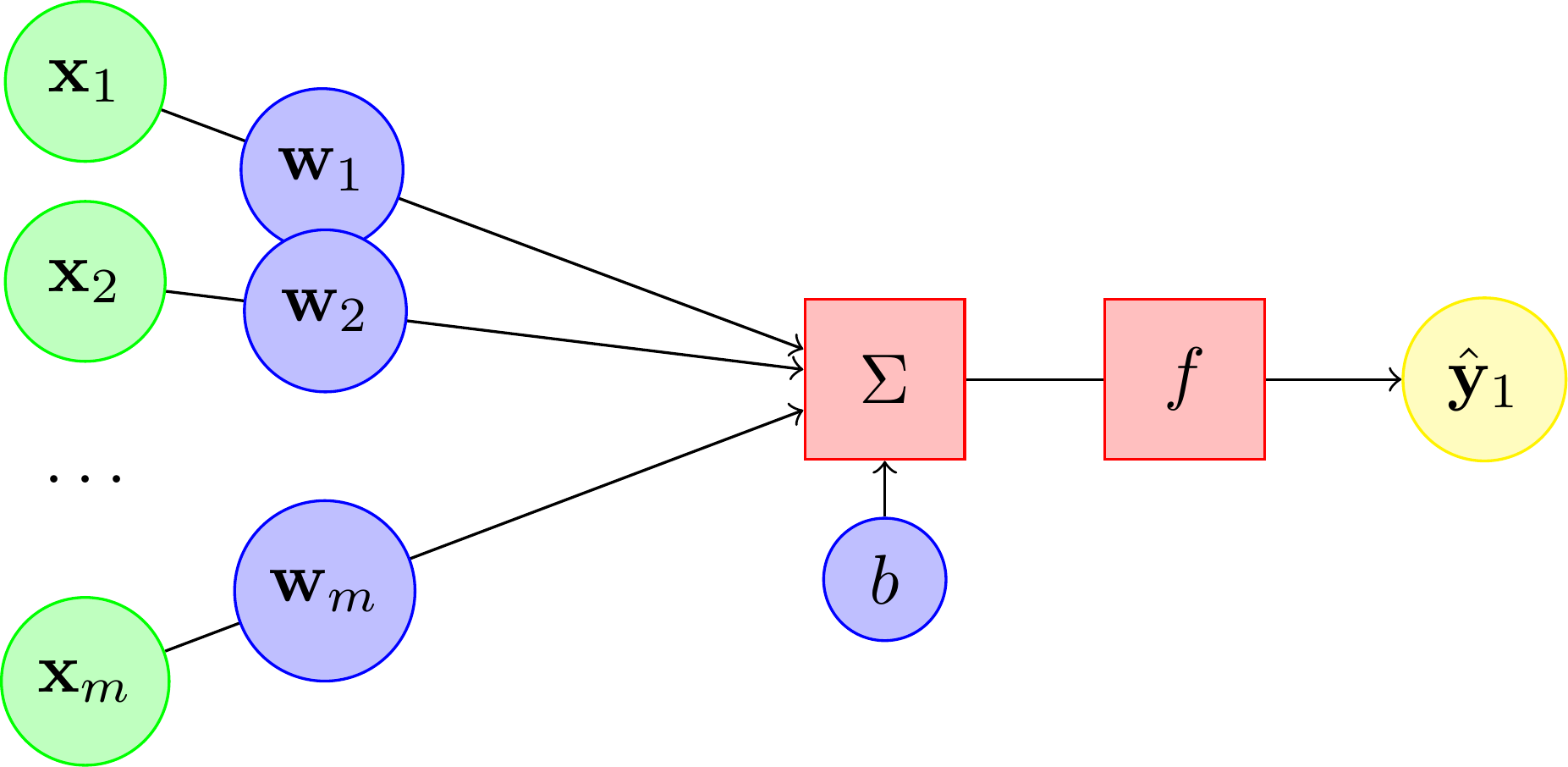
the output \(y\) is a non linear function of the inputs \(\mathbf{x}\)
Components:
Inputs \(\mathbf{x}\):
Represents the features or signals fed into the neuron.
\(\mathbf{x} = [x_1, x_2, \ldots, x_p]\)
Weights \(\mathbf{w}\):
Each input is multiplied by a weight that signifies its importance.
\(\mathbf{w} = [w_1, w_2, \ldots, w_p]\)
Bias \(\alpha_0\):
An additional parameter added to the weighted sum of inputs.
It allows the model to fit the data better by shifting the activation function.
Activation Function \(f\):
A function applied to the weighted sum of inputs and bias to produce the neuron’s output.
Common functions include
sigmoid,tanh, andReLU(Rectified Linear Unit).
Functionality:
Weighted Sum:
Compute the linear combination of inputs and weights plus the bias.
\(z = \mathbf{w} \cdot \mathbf{x} + \alpha_0 \)
Where \(z\) is the weighted sum.
Activation:
Apply the activation function to the weighted sum to get the output.
\( y = f(z) \)
Where \(y\) is the output of the neuron.
Activation Functions:
Sigmoid: \(f(z) = \frac{1}{1 + e^{-z}}\)
Tanh: \(f(z) = \tanh(z) \)
ReLU: \(f(z) = \max(0, z) \)
7.6.2. Artificial neuron model: learning phase#
In an artificial neuron model, the coefficients \(w_i\) (weights) and \(\alpha_0\) (bias) are obtained by minimizing an error function \( Err \) using a learning dataset.
Objective:
The goal is to find the optimal values for the weights \(w_i\) and the bias \(\alpha_0\) that minimize the difference between the predicted output \(\hat{y}\) and the actual target value \(y_{pred}\).
Error Function:
The error (or loss) function quantifies the discrepancy between the predicted values and the actual values. Commonly used error functions include:
Mean Squared Error (MSE):
\[ Err = \frac{1}{N} \sum_{i=1}^N (y_{pred,i} - \hat{y}_i)^2 \]where \(N\) is the number of samples, \(y_{pred,i}\) is the predicted value, and \(\hat{y}_i\) is the actual value.
Minimization of Error:
To find the optimal weights \(w_i\) and bias \(\alpha_0\), the error function is minimized using optimization algorithms. These algorithms adjust the weights and bias to reduce the error. A popular optimization method is gradient descent.
Gradient Descent:
Compute Gradient:
Calculate the gradient of the error function with respect to each weight \(w_i\) and the bias \(\alpha_0\).
The gradient gives the direction and magnitude of the steepest increase in error, so we move in the opposite direction to reduce the error.
Update Weights and Bias:
Adjust the weights and bias using the computed gradients and a learning rate \(\beta\):
\[w_i = w_i - \beta \frac{\partial Err}{\partial w_i}\]\[\alpha_0 = \alpha_0 - \beta \frac{\partial Err}{\partial \alpha_0}\]Here, \(\beta\) is the learning rate that controls the size of the steps taken in the direction of the negative gradient.
Iterate:
Repeat the gradient computation and weight/bias updates until the error function converges to a minimum or until a specified number of iterations is reached.
Summary:
In summary, the coefficients \(w_i\) and \(\alpha_0\) are optimized by minimizing the error function \(Err\), which measures the difference between the predicted values \(\hat{y}\) and the actual values \(y_{pred}\). This is achieved through iterative optimization techniques such as gradient descent.
7.6.3. Neural network#
In neural networks, each layer is composed of multiple neurons that perform specific functions.
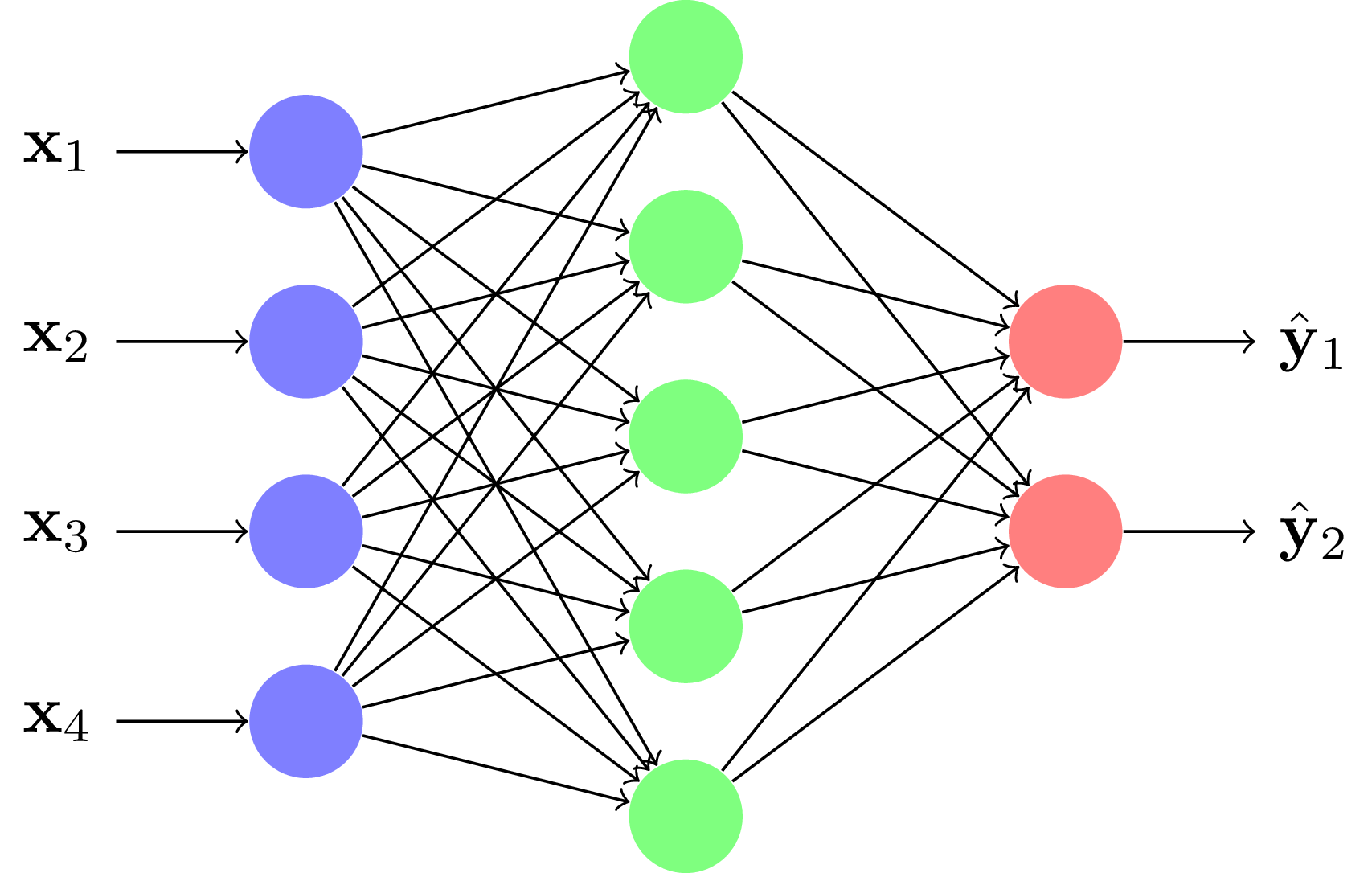
Overview of different types of layers in a neural network
Input Layer
Function: Receives the raw data (features) from the data set.
Characteristics: Each neuron in the input layer corresponds to a feature in the data set. The number of neurons in this layer is equal to the number of features.
Hidden Layers
Hidden layers are where the majority of the computations occur. They transform the inputs from the previous layer into something that can be used by the next layer. Each hidden layer consists of multiple neurons.
Fully Connected (Dense) Layer
Function: Each neuron is connected to every neuron in the previous layer.
Activation: Common activation functions include ReLU (Rectified Linear Unit), Sigmoid, or Tanh.
Example: In a dense layer with
nneurons, each neuron receives inputs from allpneurons in the previous layer, applies weights and biases, and then passes the result through an activation function.
Convolutional Layer
Function: Applies convolutional operations to the input to detect local patterns such as edges in images.
Characteristics: Uses a set of filters or kernels that convolve over the input. Each filter produces a feature map, which is a transformed version of the input data.
Activation: Typically followed by activation functions like ReLU.
Pooling Layer
Function: Reduces the spatial dimensions (width and height) of the input, thereby reducing the number of parameters and computation.
Types: Common types include Max Pooling and Average Pooling.
Max Pooling takes the maximum value in each patch of the feature map.
Dropout Layer
Function: Prevents overfitting by randomly setting a fraction of input units to zero during training.
Characteristics: Helps to ensure that the model does not rely too heavily on any one neuron or feature.
Output Layer
Function: Produces the final prediction or classification result.
Characteristics: The number of neurons in the output layer depends on the type of problem:
Regression: Typically one neuron with a linear activation function.
Binary Classification: One neuron with a sigmoid activation function.
Multiclass Classification: Multiple neurons (one per class) with a softmax activation function.
Layer Connections:
Dense Layer: Each neuron in the hidden layer connects to every neuron in the input layer and each neuron in the output layer.
Convolutional Layer: Applies a filter to local regions of the input, producing feature maps.
Pooling Layer: Reduces the dimensions of the feature maps from the convolutional layer.
Summary:
In a neural network, each layer plays a distinct role in processing data. The input layer feeds data into the network, hidden layers transform and abstract features, and the output layer produces the final prediction. Layers can vary in function and complexity, such as convolutional layers for image data, recurrent layers for sequential data, and dropout layers to mitigate overfitting.
7.6.4. Recurrent Neural Network RNN#
Recurrent Neural Networks (RNNs) are a class of neural networks designed to handle sequential data, such as time series, natural language, or any other type of data where the order of the inputs is important. Unlike traditional feedforward neural networks, RNNs have connections that form directed cycles, allowing them to maintain a form of memory about previous inputs.
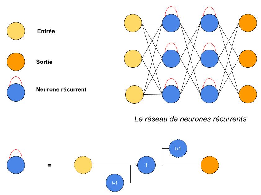
Key Concepts
Sequential Data:
RNNs are particularly useful for tasks where data points are not independent but rather dependent on previous points. For example, in language modeling, the prediction of the next word depends on the previous words.
Hidden State:
RNNs maintain a hidden state \(h_t\) that captures information from previous time steps. This hidden state is updated at each time step and is used to influence the output and the state at the next time step.
Architecture
Basic RNN Structure:
Input: A sequence of data points \(\{x_1, x_2, \ldots, x_T\}\), where \(T\) is the length of the sequence.
Hidden Layer: At each time step \(t\), the hidden state \(h_t\) is updated based on the previous hidden state \(h_{t-1}\) and the current input \(x_t\):
\[h_t = f(W_h h_{t-1} + W_x x_t + b_h)\]where \(W_h\) is the weight matrix for the hidden state, \(W_x\) is the weight matrix for the input, \(b_h\) is the bias, and \(f\) is an activation function (commonly \(\tanh\) or
ReLU).Output Layer: The output \(y_t\) at each time step can be computed from the hidden state:
\[y_t = W_y h_t + b_y\]where \(W_y\) is the weight matrix for the output and \(b_y\) is the bias.
Training:
RNNs are trained using algorithms like Backpropagation Through Time (BPTT), which extends backpropagation to handle the temporal dimension by unfolding the network over time.
7.6.5. Problematic with the RNN#
A simple classic recurrent neural network (RNN) consists of a recurrent layer followed by a dense (fully connected) layer.
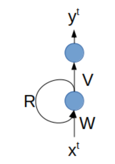
Recurrent Neural Networks (RNNs) involve a specific set of weight matrices and face particular challenges during training due to their recurrent nature.
Weight Matrices in an RNN
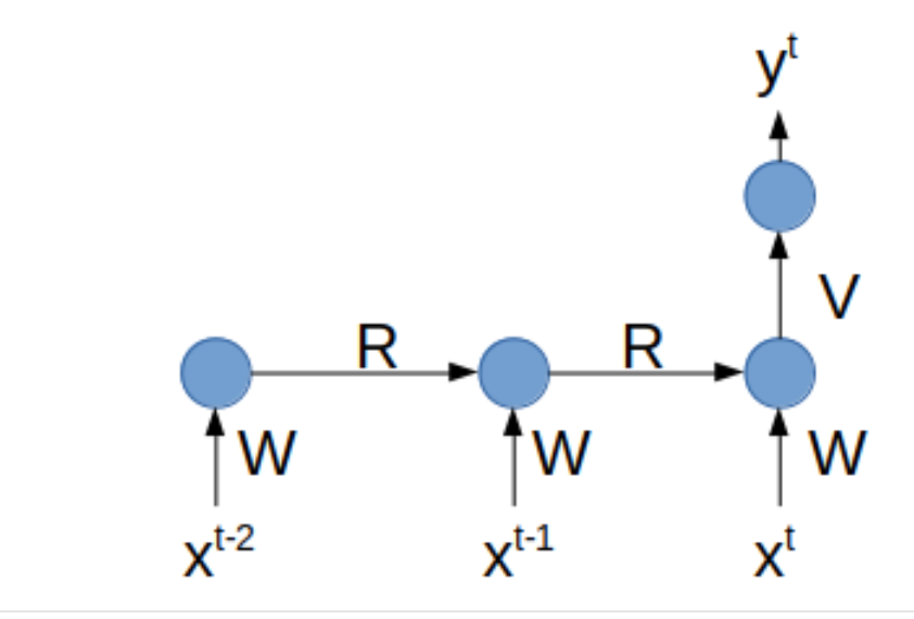
Weight Matrix \(W\):
This matrix is associated with the input layer and connects the input features to the hidden states.
Recurrent Weight Matrix \(R\):
This matrix connects the hidden state at the previous time step to the hidden state at the current time step. It captures the temporal dependencies in the sequence.
Output Weight Matrix \(V\):
This matrix connects the hidden state to the output layer, producing the final predictions or outputs.
During training, the goal is to learn the optimal values for these three weight matrices (\(W\), \(R\), and \(V\)) using a set of labeled examples.
Training Challenge with Gradient Descent
Gradient Descent:
The standard gradient descent algorithm for training neural networks is called backpropagation. It involves propagating the gradient of the error backward through the network layers, from the output layer to the input layer.
Issue with Cycles in RNNs:
The presence of the recurrent weight matrix \(R\) introduces cycles in the computation graph. When applying gradient descent, these cycles can lead to difficulties, such as:
Vanishing Gradients: Gradients may become exceedingly small as they are propagated back through many time steps, making it difficult for the network to learn long-term dependencies.
Exploding Gradients: Gradients can also become excessively large, leading to unstable training.
Summary
An RNN consists of three key weight matrices: (W) for the input layer, (R) for the recurrent connections, and (V) for the output layer. Training these networks involves learning these matrices using gradient descent. However, the recurrent nature of RNNs introduces cycles, complicating the backpropagation process. This issue is addressed through techniques like backpropagation through time (BPTT), though challenges such as vanishing and exploding gradients remain. Advanced architectures, such as LSTMs and GRUs, are often used to overcome these challenges and improve the performance of RNNs on sequential tasks.
7.6.6. Back propagation Through Time (BPTT)#
Backpropagation Through Time (BPTT):
In the case of RNNs, this concept is extended to handle sequences. This approach, known as back propagation through time, involves unfolding the RNN through the time steps \(K\) times (\(K\) = number of internal hidden state from 2 to 100) and applying back propagation to this unfolded structure. See figure for \(K=2\)
BPTT with Cyclic Dependencies:
While BPTT is designed to handle the unfolding of RNNs, the recurrent connections can still present challenges. Proper implementation involves:
Carefully managing the unfolding process to ensure that the gradients are correctly propagated through the cycles.
Using techniques to mitigate the vanishing and exploding gradient problems, such as gradient clipping or using advanced RNN architectures like LSTM or GRU, which are designed to address these issues.
Attention
In Recurrent Neural Networks (RNNs), training challenges related to gradients are significant due to the nature of their architecture. Two main issues are particularly noteworthy: vanishing gradients and exploding gradients.
Vanishing Gradients
Issue:
As RNNs are unfolded through time steps, they become very deep, creating a long chain of layers. This depth can lead to the vanishing gradient problem, where gradients become exceedingly small as they are back propagated through many time steps.
This problem makes it difficult for the network to learn long-term dependencies because the error signal diminishes as it propagates back through the network, especially affecting lower layers or earlier time steps.
Strategies to Mitigate Vanishing Gradients:
Batch Normalization: This technique normalizes the inputs of each layer to improve the training speed and stability.
Dropout: Regularly dropping units (along with their connections) during training to prevent overfitting and make the network more robust.
Regularization (L1 and L2): Adding regularization terms to the loss function to prevent overfitting and control the complexity of the model.
Use of Advanced RNN Architectures: Incorporating architectures like Long Short-Term Memory (LSTM) or Gated Recurrent Units (GRU) that are specifically designed to handle vanishing gradients by incorporating gating mechanisms that control the flow of information.
Exploding Gradients
Issue:
Exploding gradients occur when the gradients become excessively large, leading to very large updates to the weights. This can destabilize the training process and lead to extremely high weights that make the model’s performance erratic.
Solution:
Gradient Clipping: This technique involves setting a threshold value for the gradient norm. If the norm of the gradient exceeds this threshold, it is scaled down to a predefined maximum value. This helps in preventing gradients from growing too large and causing instability.
7.6.7. Advanced RNN Variants#
To address the limitations of basic RNNs, several advanced architectures have been developed:
Long Short-Term Memory (LSTM) Networks:
Architecture: LSTMs introduce special units called memory cells that maintain information over long periods. They use gates (input, output, and forget gates) to control the flow of information into and out of the memory cells.
Advantages: LSTMs are effective at learning long-term dependencies and mitigating the vanishing gradient problem.
Gated Recurrent Units (GRUs):
Architecture: GRUs are a simplified version of LSTMs with fewer gates. They use a reset gate and an update gate to control the flow of information.
Advantages: GRUs often perform similarly to LSTMs but with less computational complexity.
7.6.8. LSTM : Long Short Term Memory#
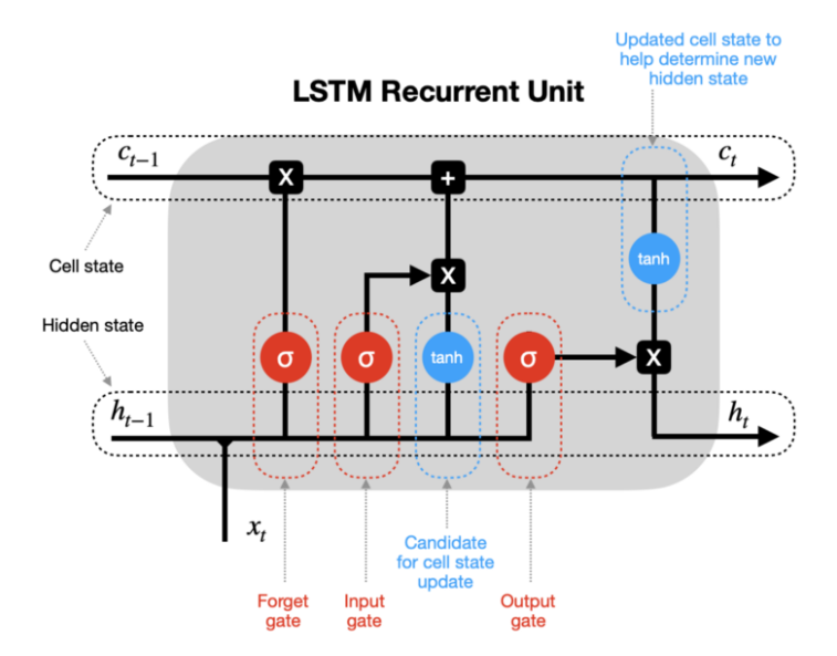
To model long-term dependencies, it is essential to enable Recurrent Neural Networks (RNNs) to maintain state over extended periods. This is the goal of Long Short-Term Memory (LSTM) cells, which are specifically designed to address this need.
LSTM cells are a type of RNN architecture that include mechanisms to preserve information over long sequences.
Key Components of LSTM Cells
Cell State (or Memory Cell):
The cell state is a crucial component of LSTM cells. It serves as a long-term memory that can retain information over many time steps. This state allows the network to maintain relevant information for extended periods, addressing the issue of vanishing gradients often encountered in standard RNNs.
Gates:
LSTM cells use gates to control the flow of information into and out of the cell state. These gates are learned during training and regulate how much of the past information should be remembered or forgotten.
Forget Gate:
The forget gate decides what portion of the previous cell state should be discarded. It uses a sigmoid activation function to output a value between 0 and 1, indicating how much of each component of the cell state should be kept or thrown away.
Input Gate:
The input gate determines how much of the new information should be added to the cell state. It also uses a sigmoid function to decide which values will be updated, combined with a tanh function to create candidate values that can be added to the cell state.
Output Gate:
The output gate controls the output of the cell state. It decides which parts of the cell state will be output to the next layer and uses a sigmoid function to filter this output, combined with a tanh function to adjust the values accordingly.
How LSTM Cells Work
Update Cell State:
At each time step, the forget gate decides which information from the previous cell state should be retained.
The input gate updates the cell state with new information based on the current input and the previous hidden state.
The cell state is updated accordingly, incorporating both retained and new information.
Generate Output:
The output gate processes the updated cell state and produces the final output of the LSTM cell. This output is used for predictions or fed into subsequent layers.
By incorporating these mechanisms, LSTM cells effectively manage long-term dependencies, allowing RNNs to maintain relevant information over many time steps and improving their performance on tasks requiring memory of past events.
Summary of LSTM
LSTM cells are designed to address the limitations of traditional RNNs by providing a mechanism to maintain long-term dependencies. They do this through:
A cell state (memory) that retains information over long periods.
Gates (forget, input, and output) that regulate the flow of information into, out of, and within the cell state.
These features make LSTMs powerful for tasks involving sequences with long-term dependencies, such as language modeling, time series prediction, and more.
7.7. Implementation and usage#
7.7.1. RandomForest algorithm#
Python library
scikit learn
from sklearn.linear_model import LinearRegression
from sklearn.ensemble import RandomForestRegressor
from sklearn.neighbors import KNeighborsRegressor
from sklearn.metrics   import r2_score
# choix de l'algorithme
clf = RandomForestRegressor()
#clf = KNeighborsRegressor()
#clf = LinearRegression()
Xlearn = X.copy()
ylearn = y[:,0]
clf.fit(Xlearn,ylearn);
print("score = {:2d}%".format(int(100*clf.score(Xlearn, ylearn))))
yp = clf.predict(Xlearn)
print("R2 = {:3.2f}%".format(r2_score(ylearn,yp)))
score = 99%
R2 = 1.00%
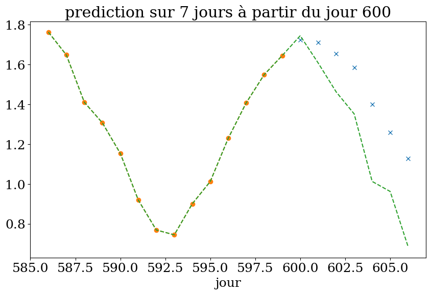
def plot_pred():
    plt.figure(figsize=(10,6))
    plt.plot(Ts[t2:t2+nap],ypred,'x')
    plt.plot(Ts[t2-nav:t2],Xpred[0],'--o')
    plt.plot(Ts[t2-nav:t2+nap],ys[t2-nav:t2+nap],'--')
    plt.xlabel("jour")
    plt.title(f"prediction sur {nap} jours à partir du jour {t2}");
    return
# prediction à partir de t2
t2 = t0
Xpred  = np.array([ys[t2-nav:t2]])
ypred  = np.zeros(nap)
Xp     = Xpred.copy()
ypred[0] = clf.predict(Xp)[0]
for i in range(1,nap):
    Xp[0,:-i] = Xpred[0,i:]
    Xp[0,-i:] = ypred[:i]
    ypred[i] = clf.predict(Xp)[0]
Xpred.shape, ypred.shape
((1, 14), (7,))
plot_pred()
7.7.2. Implementation and usage of LSTM RNN#
Python library KERAS
tensor flow Keras RNN
#Machine learning
from sklearn import preprocessing
import tensorflow as tf
import statsmodels as st
from statsmodels.tsa.seasonal import STL
from sklearn.model_selection  import train_test_split
Xlearn = X.copy()
ylearn = y.copy()
Xlearn = Xlearn.reshape(X.shape[0], nav, 1)
ylearn = ylearn.reshape(y.shape[0], nap, 1)
Xlearn.shape, ylearn.shape
((400, 14, 1), (400, 7, 1))
#Nombre d'époque d'entrainement (fenetre de taille nav)
#EPOQUE = 300
EPOQUE = 200
#EPOQUE = 50
# modèle du réseaux de neurones(4 rangées (100,100,50,50) dont la première LSTM)
# si pas activation: activation='linear' lineaire a(x)=x, sinon test avec 'relu'
modele_lstm = tf.keras.models.Sequential([
    tf.keras.layers.LSTM(nav),
    tf.keras.layers.Dense(nav,activation='tanh'),
    tf.keras.layers.Dense(nap,activation='tanh'),
    tf.keras.layers.Dense(nap)
])
#Configuration du modèle(on minimise avec la méthode des moindres carrés)
modele_lstm.compile(optimizer='adam', metrics=['mae'], loss='mse')
print(EPOQUE)
200
#Lance l'entrainement du modèle
import time
time_start = time.time()
modele_lstm.fit(Xlearn, ylearn, epochs=EPOQUE, verbose = False)
print('phase apprentissage: {:.2f} seconds'.format(time.time()-time_start))
phase apprentissage: 11.87 seconds
modele_lstm.summary()
Model: "sequential"
_________________________________________________________________
 Layer (type)                Output Shape              Param #
=================================================================
 lstm (LSTM)                 (None, 14)                896

 dense (Dense)               (None, 14)                210

 dense_1 (Dense)             (None, 7)                 105

 dense_2 (Dense)             (None, 7)                 56

=================================================================
Total params: 1,267
Trainable params: 1,267
Non-trainable params: 0
_________________________________________________________________
ypred = modele_lstm.predict(Xlearn, verbose=False)
print(Xlearn.shape,ypred.shape)
Ylearn = ylearn.reshape(ylearn.shape[0],nap,)
print("R2 score {:.2f}".format(r2_score(Ylearn, ypred)))
print("model evaluate loss/mae")
modele_lstm.evaluate(Xlearn,ylearn)
(400, 14, 1) (400, 7)
R2 score 0.98
model evaluate loss/mae
13/13 [==============================] - 0s 1ms/step - loss: 0.0120 - mae: 0.0867
[0.011985886842012405, 0.0866922065615654]
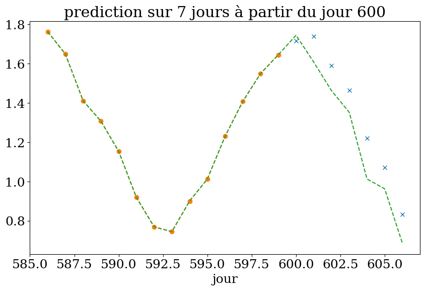
# prediction à partir de t2
t2 = t0
Xpred  = np.array([ys[t2-nav:t2]]).reshape(1,nav,1)
ypred = modele_lstm.predict(Xpred, verbose=True)
print(Xpred.shape,ypred.shape)
1/1 [==============================] - 0s 14ms/step
(1, 14, 1) (1, 7)
Xpred = Xpred.reshape(1,nav,)
ypred = ypred.reshape(nap)
plot_pred()
7.8. Application: Meteorological prediction#
TP3_meteonet_prediction.ipynb
