5. Algorithms for AI/ML#
Marc Buffat dpt mécanique, université Lyon 1
%matplotlib inline
import sys
import numpy as np
import matplotlib.pyplot as plt
# police des titres
plt.rc('font', family='serif', size='18')
from IPython.display import display,Markdown
import sklearn as sk
#sys.path.insert(1,"/home/cours/DatabaseIA")
from datasetIA import *
5.1. Problematic of the machine learning#
objective : prediction of the function \(\mathcal{F}\) s.t.
using a learning data set \(\textbf{X}_i, Y_i\)
\(\rightarrow\) Minimization problem
Find the best approximation \(\mathbf{F}\) that minimizes the error \(J\) over the learning data set.
\(J\) is a cost function, for example:
\(\mathbf{F}(\mathbf{X}_i)\) is a function of a linear combination of the data \(X_i\)
there is no explicit form for \(\mathbf{F}\) that depends of a large number of parameters to be determined by a minimization method
Implicit Algorithm that needs an annotated data-set for the learning and the validation phase (supervised machine learning)
5.1.1. Choice of algorithms#
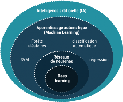
no universal algorithm (even neural networks)
5.1.1.1. choice of the minimization method#
local method:
exact gradient: gradient method, Newton’s method, Conjugate gradient method.
approximation of the gradient: Stochastic Gradient Descent, mini batch method
without gradient: simplex method
global method:
stochastic: Simulated annealing, Differential evolution, Genetic algorithms.
5.1.1.2. representation of the function F#
- combination of functions
- no simple explicit expression
5.1.2. Application domains of machine learning#
Data base Processing (experimental or numerics)
Modelization
Big Data
ATTENTION
it’s not the solution for all problems
classical methods / semi-analytical
to be used wisely
5.2. Basic Algorithms#
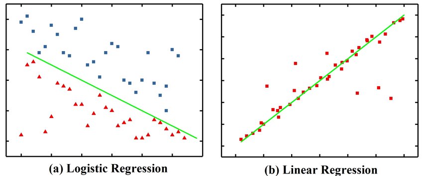
Regression: logistic (classification) or linear (prediction)
5.2.1. Linear Regression#
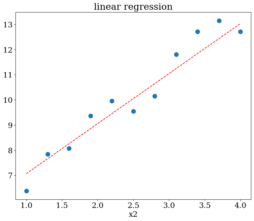
Linear regression by least squares
The Linear Regression fits a linear model
with the coefficients:
to minimize the residual sum of squares between the observed targets in the dataset and the targets predicted by the linear approximation (least squares method).
scikit learn model: LinearRegression
from sklearn.linear_model import LinearRegression

N = 11
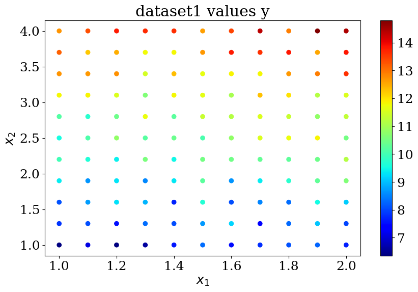
X,y = dataset1(N)
reg = LinearRegression().fit(X, y)
print("score = {:2d}%".format(int(100*reg.score(X, y))))
print("loi lineaire y = {:.2f} +  {} X".format(reg.intercept_,reg.coef_))
score = 91%
loi lineaire y = 4.08 +  [0.9950683  1.98990227] X
plot_data1(X,y,"dataset1 values y")
# prediction en x2=1
Xpred  = np.array([[1,x] for x in np.linspace(1,4,21) ])
ypred  = reg.predict(Xpred)
plot1(N,X,y,Xpred,ypred,titre="linear regression")
5.2.2. Logistic Regression#
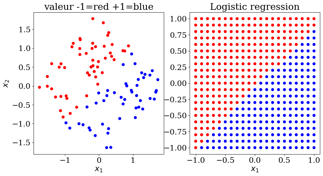
Logistic regression, despite its name, is a linear classification model rather than a regression model. Logistic regression is also known in the literature as logic regression, maximum entropy classification (MaxEnt), or log-linear classifier. In this model, the probabilities describing the possible outcomes of a single trial are modeled using a logistic function.
Logistic regression is a simple and efficient classification algorithm that does not require significant computational power and is easy to implement. This learning model is widely used by data analysts and scientists.
scikit learn model: LogisticRegression
Logistic regression is implemented in LogisticRegression. This implementation can fit binary logistic regression, One-vs-Rest, or multinomial logistic regression with optional regularization (l1, l2, elastic net, none)
Logistic regression algorithm
Logistic regression is a statistical method for predicting binary classes. The outcome or target variable is dichotomous in nature, meaning there are only two possible classes. It calculates the probability of an event occurring.
It is a special case of linear regression where the target variable is categorical. It uses a log of odds as the dependent variable. Logistic regression predicts the probability of occurrence of a binary event using a logit function:
linear regression equation
sigmoid function $\( p = \frac{1}{1+e^{-z}} \)$
Probability y=1 $\( p = \frac{1}{1+e^{-(\beta_0 + \beta_1 X_1 + ... + \beta_n X_n)}}\)$
Limit
Logistic regression is not suitable for a large number of applications. This algorithm cannot solve the problem of non-linearity, which requires the transformation of non-linear features.
Thus, logistic regression does not work well with independent variables that are not correlated with the target variable and are very similar to each other.
from sklearn.linear_model import LogisticRegression

N = 10
X,y,col = dataset2(N)
clf = LogisticRegression(random_state=0).fit(X, y)
print("score = {:2d}%".format(int(100*clf.score(X, y))))
score = 98%
# prediction
NN = 21
Xpred, ypred, colpred = predict2(NN,clf.predict)
plot2(X,col, Xpred,colpred, titre="Logistic regression")
5.2.3. Decision Trees#
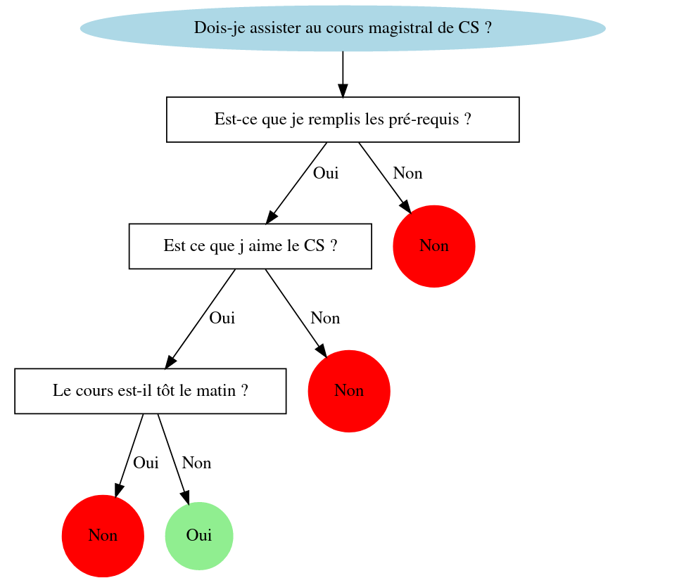
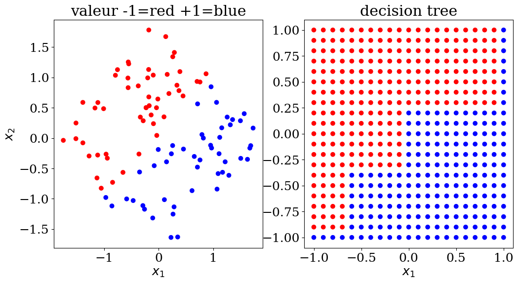
To make a prediction, decision trees use a set of “If Then Else” decision rules on the features (data). This method allows the decomposition of a dataset into increasingly smaller subsets. The final subsets can then be assigned a class (0 or 1 for binary classification). The goal of the model is to create homogeneous subsets (containing examples of the same class) to minimize the error of its predictions.
classification
scikit learn model
DecisionTreeClassifier
regression
scikit learn model
DecisionTreeRegressor
Problem: The result depends on the order of the questions !
5.2.3.1. Decision tree: classification#
scikit learn DecisionTreeClassifier
from sklearn.tree import DecisionTreeClassifier

N = 10
X,y,col = dataset2(N)
clf = DecisionTreeClassifier()
clf = clf.fit(X, y)
print("score = {:2d}%".format(int(100*clf.score(X, y))))
score = 100%
# prediction
NN = 21
Xpred, ypred, colpred = predict2(NN, clf.predict)
plot2(X,col, Xpred,colpred,titre="decision tree")
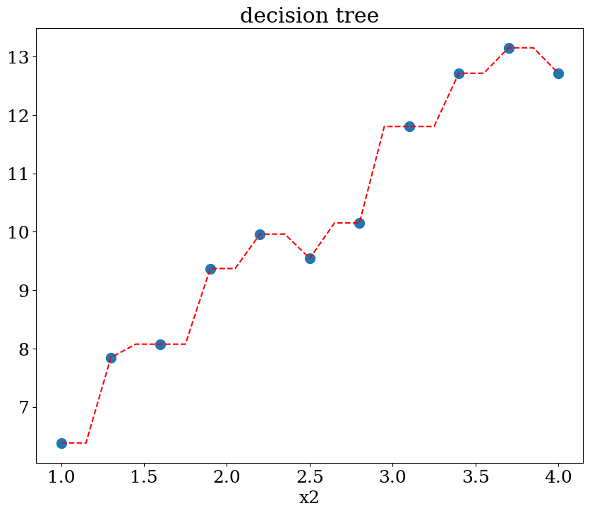
5.2.3.2. Décision tree: régression#
scikit learn DecisionTreeRegressor
from sklearn.tree import DecisionTreeRegressor

N = 11
X,y = dataset1(N)
clf = DecisionTreeRegressor()
clf = clf.fit(X, y)
print("score = {:2d}%".format(int(100*clf.score(X, y))))
score = 100%
# prediction en x2=1
NN = 51
Xpred  = np.array([[1,x] for x in np.linspace(1,4,21) ])
ypred  = clf.predict(Xpred)
plot1(N,X,y, Xpred,ypred,titre="decision tree")
5.2.4. Random forest algorithm#
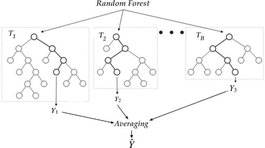
Random Forest models consist of multiple Decision Trees (a “forest” of decision trees). The result returned by a Random Forest is the majority class output by the individual Decision Trees that compose it. Each of these Decision Trees is trained with a random sample of the training data and a random subset of the features.
5.2.4.1. Random forest classification#
scikit learn RandomForestClassifier
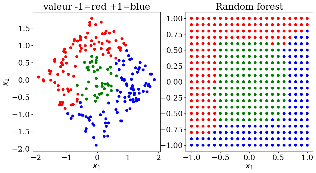
use of a data-set dataset3 with 3 sets of values (-1,0,+1)
influence of the parameters:
max_depth (of the tree) 2, 3 or None
from sklearn.ensemble import RandomForestClassifier

N=15
X,y,col = dataset3(N)
clf = RandomForestClassifier(max_depth=None, random_state=0)
cfl = clf.fit(X, y)
print("score = {:2d}%".format(int(100*clf.score(X, y))))
score = 100%
# prediction
NN = 21
Xpred,ypred,colpred = predict3(NN, clf.predict)
plot3(X,col, Xpred,colpred, titre="Random forest")
5.2.4.2. Random forest régression#
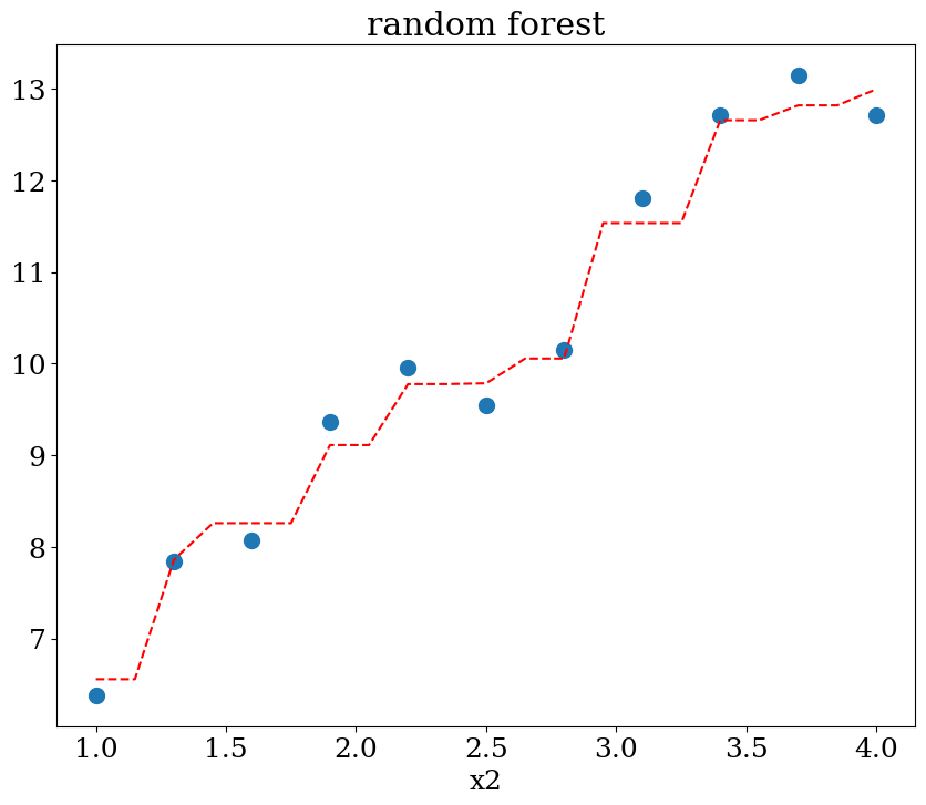
scikit learn RandomForestRegression
influence of the parameters:
max_depth (of the trees) 2, 3 ou None
from sklearn.ensemble import RandomForestRegressor

N=11
X,y = dataset1(N)
clf = RandomForestRegressor(max_depth=None, random_state=0)
cfl = clf.fit(X, y)
print("score = {:2d}%".format(int(100*clf.score(X, y))))
score = 98%
NN = 51
Xpred  = np.array([[1,x] for x in np.linspace(1,4,21) ])
ypred  = clf.predict(Xpred)
plot1(N,X,y, Xpred,ypred,titre="random forest")
5.2.5. K Nearest Neighbors (KNN)#
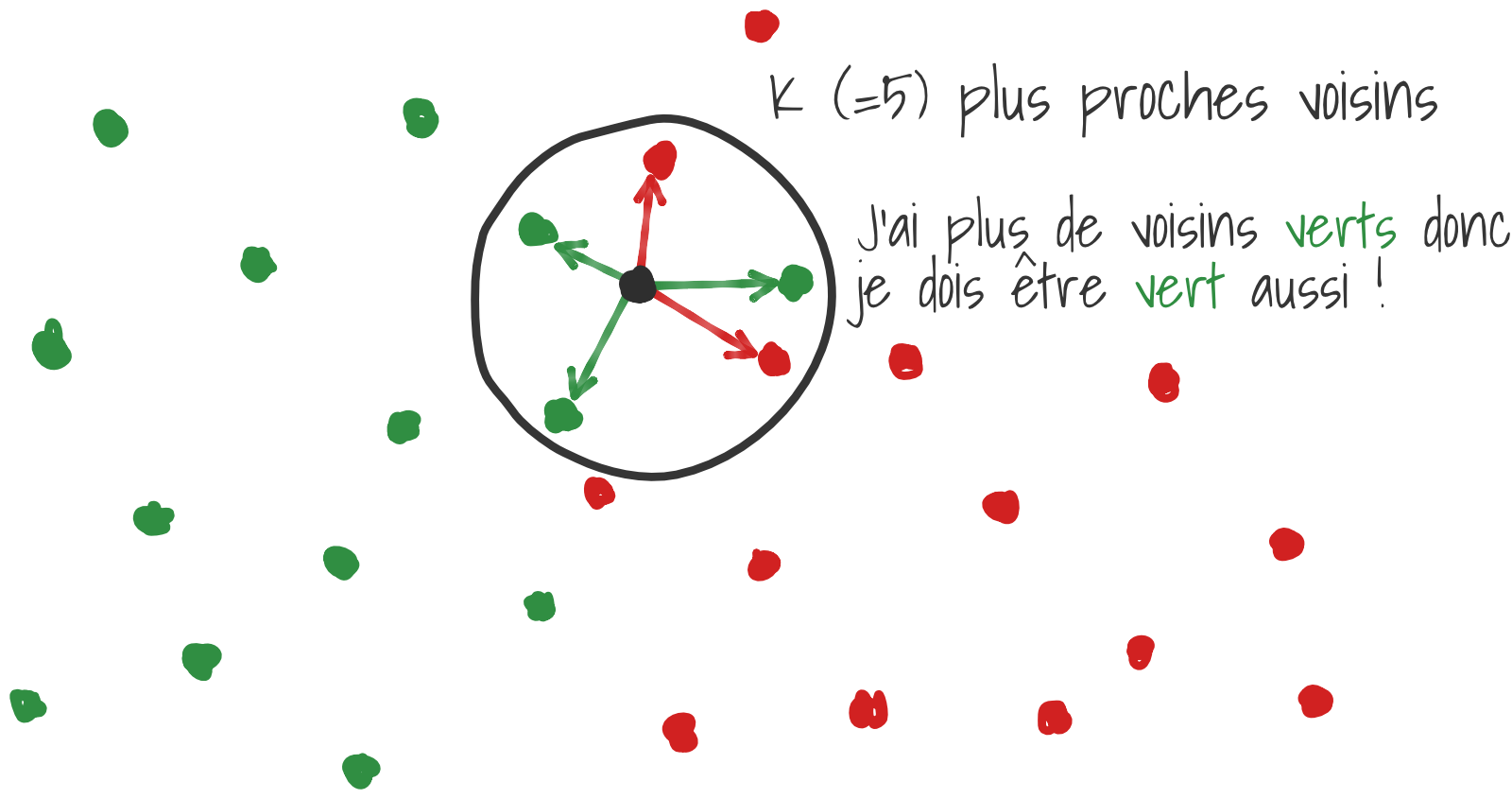
KNN (K-Nearest Neighbors) is a classification algorithm where the class of a data point is determined based on the classes of its K nearest neighbors. The algorithm works by finding the K closest data points to the target point and assigning the most common class among these neighbors to the target point. It’s a simple, instance-based learning method that does not require explicit training but relies on the distance metric to make predictions.
The KNN algorithm assigns a class to an example based on the majority class among its K nearest neighbors. K is a parameter that needs to be optimized by the user; it is generally preferable to choose an odd value for K in binary classification to avoid ties. The Euclidean distance between two feature vectors is commonly used to calculate the proximity between two examples.
5.2.5.1. KNN classification#
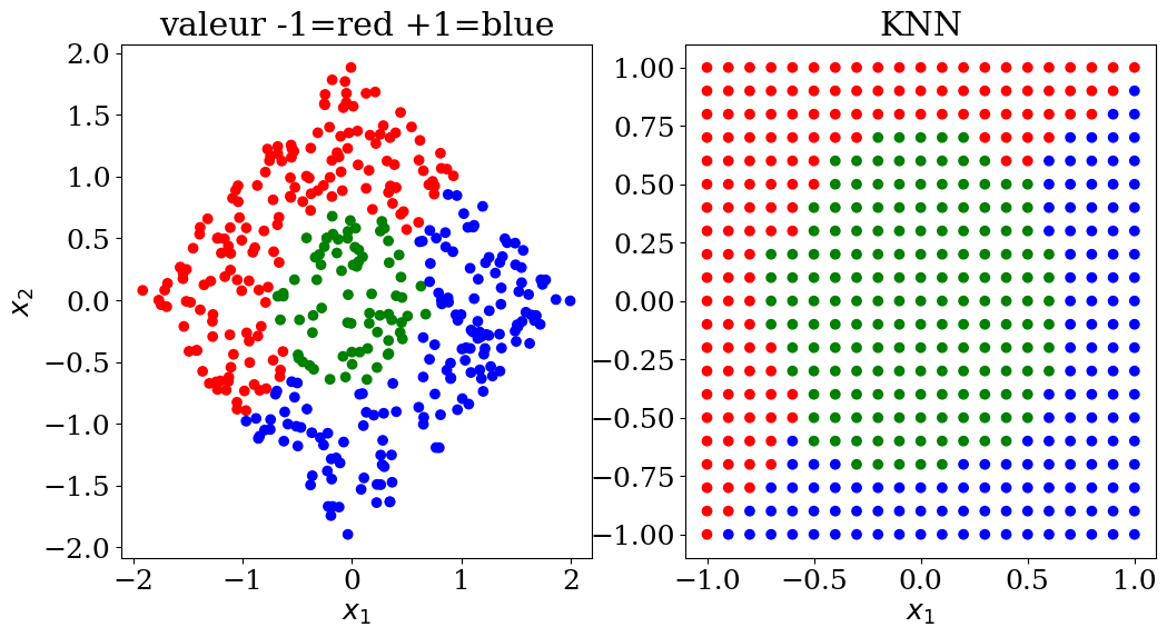
scikit learn KNeighborsClassifier
parameters:
n_neighbors = 2,3,..5
from sklearn.neighbors import KNeighborsClassifier

N = 20
X,y,col = dataset3(N)
neigh = KNeighborsClassifier(n_neighbors=5)
neigh = neigh.fit(X, y)
print("score = {:2d}%".format(int(100*neigh.score(X, y))))
score = 98%
# prediction
NN = 21
Xpred,ypred,colpred = predict3(NN, neigh.predict)
plot3(X,col, Xpred,colpred, titre="KNN")
5.2.5.2. KNN regression#
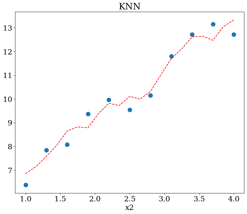
scikit learn KNeighborsRegressor
parameters:
n_neighbors = 2,3,..5
from sklearn.neighbors import KNeighborsRegressor

N=11
X,y = dataset1(N)
neigh = KNeighborsRegressor(n_neighbors=5)
neigh = neigh.fit(X, y)
print("score = {:2d}%".format(int(100*neigh.score(X, y))))
score = 93%
NN = 51
Xpred  = np.array([[1,x] for x in np.linspace(1,4,21) ])
ypred  = neigh.predict(Xpred)
plot1(N,X,y, Xpred,ypred,titre="KNN")
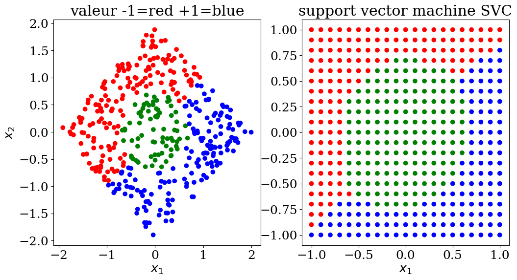
5.2.6. Support vector machine SVM#
scikit learn svm
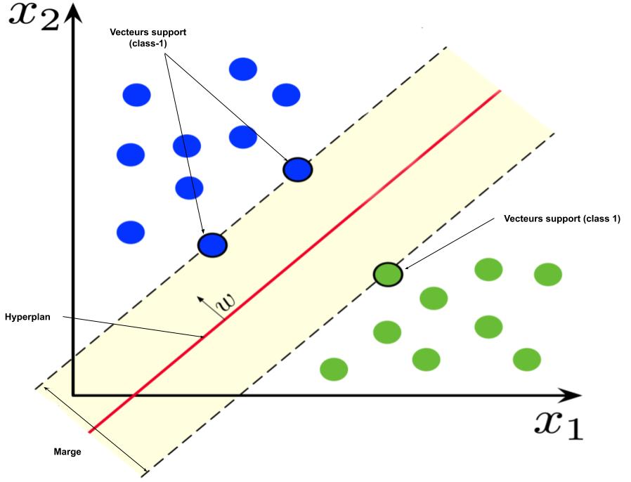
Support Vector Machines (SVM) are a set of supervised learning algorithms used for classification and regression tasks. The core idea of SVM is to find the optimal hyperplane that best separates different classes in the feature space.
Here’s a brief overview of how SVM works:
Linear Classification: For linearly separable data, SVM finds the hyperplane (a line in 2D, a plane in 3D, or a hyperplane in higher dimensions) that maximizes the margin between the two classes. The margin is the distance between the hyperplane and the nearest data points from either class, known as support vectors.
Kernel Trick: For non-linearly separable data, SVM can use a kernel function to transform the feature space into a higher dimension where a linear separation is possible. Common kernels include polynomial, radial basis function (RBF), and sigmoid.
Regularization: SVM includes a regularization parameter (C) that balances the trade-off between maximizing the margin and minimizing classification errors. A high C value aims for a smaller margin and fewer classification errors, while a low C value allows for a larger margin but may result in more misclassifications.
Support Vectors: These are the data points that lie closest to the decision boundary. They are crucial in defining the hyperplane and are the only points needed to construct the model.
SVM is known for its effectiveness in high-dimensional spaces and its flexibility due to the kernel trick. However, it can be computationally intensive for very large datasets.
from sklearn import svm

N = 20
X,y,col = dataset3(N)
clf = svm.SVC()
clf = clf.fit(X,y)
print("score = {:2d}%".format(int(100*clf.score(X, y))))
score = 99%
# prediction
NN = 21
Xpred, ypred, colpred = predict3(NN, clf.predict)
plot3(X,col, Xpred,colpred, titre="support vector machine SVC")
5.3. Neural Networks in artificial intellignece (AI)#
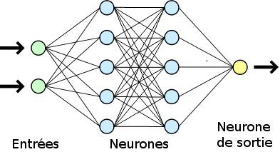
Neural networks in artificial intelligence (AI) are computational models inspired by the functioning of the human brain, designed to recognize patterns and learn complex relationships between data. Here is an overview of their main concepts and types:
Basic Concepts
Neuron: The basic unit of a neural network, similar to a nerve cell in the brain. Each neuron receives inputs, performs a computation, and produces an output.
Layer: A neural network consists of several layers:
Input Layer: Receives raw data.
Hidden Layers: Perform intermediate transformations of the data. A network can have multiple hidden layers, making it “deep” in the case of deep neural networks.
Output Layer: Provides the final prediction or classification.
Activation Function: Determines whether a neuron should be activated by applying a non-linear transformation to the data. Common functions include sigmoid, hyperbolic tangent (tanh), and ReLU (Rectified Linear Unit).
Forward Propagation: The process by which data passes through the layers of the network, from input to output, to produce a prediction.
Backpropagation: The algorithm used to train the network by adjusting the weights of the connections based on the error between the prediction and the actual value, minimized by a loss function.
5.3.1. Deep Learning#
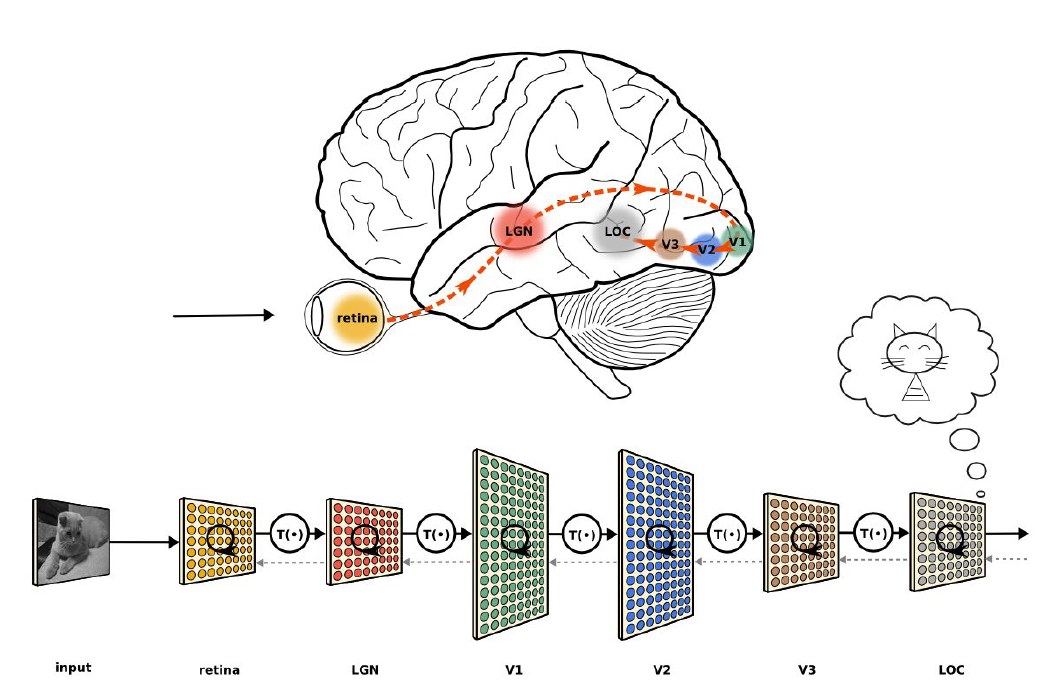
misleading analogy between neural networks and the human brain
Neural Networks vs. the Human Brain:
Imagine a neural network as a simplified version of the human brain. In this analogy:
Neurons: In a neural network, the artificial neurons are like the neurons in your brain. Both process information and make decisions based on inputs. However, unlike the intricate, highly connected neurons in the brain, artificial neurons in a network are more straightforward and mathematical.
Layers: Neural networks have layers of neurons, similar to how the brain has different layers and regions responsible for various functions. While both have layers, neural network layers are highly structured and organized, whereas the brain’s layers are far more complex and involve rich biological processes.
Activation Functions: Just as neurons in the brain fire in response to certain stimuli, artificial neurons in a neural network use activation functions to decide whether to activate based on input. In reality, brain neuron firing is influenced by a range of complex biochemical processes.
Learning: Neural networks learn by adjusting weights based on errors, akin to how the brain adjusts connections between neurons based on experience. In the brain, learning involves complex processes like neuroplasticity and involves the strengthening or weakening of synaptic connections.
Backpropagation: Neural networks use backpropagation to update weights based on errors, which is a mathematical method for learning. The brain’s learning process, while similar in that it adjusts connections, involves biochemical changes and intricate neural communication that isn’t captured by simple algorithms.
Data Processing: Neural networks process data in a structured manner with a clear path from input to output. The brain, however, processes information in a highly interconnected and dynamic way, integrating sensory inputs, emotions, and past experiences in a far more complex system.
In summary, while there are parallels between neural networks and the human brain, such as information processing and learning, the analogy is imperfect. Neural networks are mathematical models with simplified and structured components, while the brain is a complex biological system with intricate and multi-dimensional processes.
5.4. Neuron (informatique)#
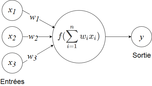
\(f\) is an activation function
Question : which activation function \(f\) should be chosen to obtain the linear model ?
5.4.1. Classical Activation Functions#
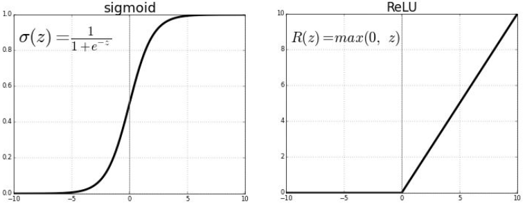
left sigmoid : To be placed at the end of a network to predict a probability (between 0 and 1)
right relu : Between each layer to introduce non-linearity (at a low computational cost)
5.4.2. Formal Neuron#
The formal neuron is a model characterized by input signals \(\mathbf{x}=[x_1,...,x_p]\) and an activation function \(f\) to compute the output \(y\).
The activation function performs a transformation of an affine combination of the input signals, where \(\alpha_0\), the constant term, is called the neuron’s bias. This affine combination is determined by a weight vector \(\mathbf{\alpha}=[\alpha_1,..\alpha_2]\) associated with each neuron, and its values are estimated during the learning phase. These weights constitute the distributed memory or knowledge of the network.
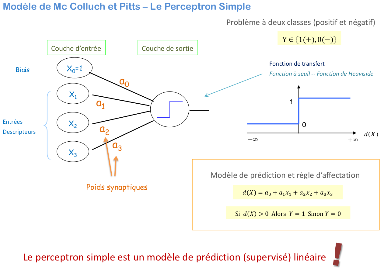
5.4.2.1. Simple perceptron model#
The Perceptron model is a fundamental algorithm in machine learning and neural networks used for binary classification. It was introduced by Frank Rosenblatt in 1957. Here’s an overview of the Perceptron model:
Key Concepts
Structure:
Inputs: The Perceptron receives input signals \(\mathbf{x} = [x_1, x_2, \ldots, x_p]\).
Weights: Each input is associated with a weight \(\mathbf{w} = [w_1, w_2, \ldots, w_p]\), which adjusts the importance of each input.
Bias: The bias term \(\alpha_0\) helps adjust the decision boundary.
Affine Combination:
The Perceptron computes a weighted sum of the inputs plus the bias:
\[ z = \mathbf{w} \cdot \mathbf{x} + \alpha_0 = w_1x_1 + w_2x_2 + \cdots + w_p x_p + \alpha_0\]
Activation Function:
The Perceptron uses a step function as its activation function:
\[\begin{split} y = \begin{cases} 1 & \text{if } z \geq 0 \\ 0 & \text{if } z < 0 \end{cases} \end{split}\]This function outputs either 1 or 0 based on whether the affine combination ( z ) is above or below a threshold (which is 0 in this case).
Learning Rule:
During the training phase, the Perceptron adjusts the weights and bias based on the errors it makes. The update rules are:
\[ w_i \leftarrow w_i + \eta \cdot (y_{\text{true}} - y_{\text{pred}}) \cdot x_i\]\[\alpha_0 \leftarrow \alpha_0 + \eta \cdot (y_{\text{true}} - y_{\text{pred}})\]Here, \(\eta\) is the learning rate, \(y_{\text{true}}\) is the actual label, and \(y_{\text{pred}}\) is the predicted label.
Training Process:
The Perceptron is trained using a supervised learning approach where it iteratively updates its weights and bias to minimize classification errors on the training dataset.
Limitations:
The Perceptron can only solve linearly separable problems. It cannot classify data that is not linearly separable (e.g., the XOR (exclusive or) problem).
Applications
The Perceptron serves as a building block for more complex neural network models, particularly in understanding the basics of linear classifiers and learning algorithms.
It is a foundational concept for further exploration into multi-layer neural networks and other machine learning techniques.
The Perceptron model provides a simple yet powerful introduction to classification algorithms and neural networks, demonstrating the core ideas of linear decision boundaries and iterative learning.
5.5. Neural networks / layers#

left : depth = 1
right : depth = 2
5.5.1. formalism: Multi Layer Perceptron (MLP)#
The Multilayer Perceptron (MLP) is a network composed of successive layers. A layer is a set of neurons that have no connections between themselves. An input layer reads the incoming signals, one neuron per input \(x_j\), and an output layer provides the system’s response \(Y\).
The pp inputs or explanatory variables of the model are denoted \(X_1,...,X_p\), while the output is the target variable \(Y\) to be predicted by the model.
Typically, in regression (where \(Y\) is quantitative), the final layer consists of a single neuron with an identity activation function, while the other neurons (in the hidden layers) use the sigmoid activation function.
This model includes non-linear “hidden” layers. The term “hidden” simply means that these layers are not directly connected to the inputs or outputs.
5.6. Learning using neural networks#
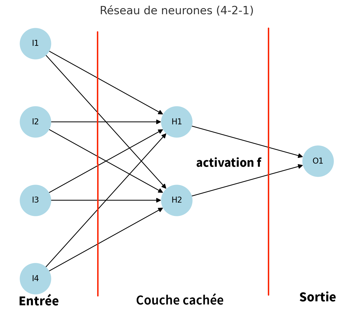
Let us consider a neural network with \(p=4\) inputs (\(I1−I4\)), one hidden layer with q=2 neurons (\(H1−H2\)), and r=1 output (\(O1\)), with an activation function \(f\) for the hidden layer and a linear output for regression.
We then have the following relations:
This model therefore depends on the following 13 parameters:
vector (2) \(\mathbf{B^1}={b^1}_{k=1,2}\)
matrix (4,2) \(\mathbf{W^1}={w^1}_{k,i}\)
vector (1) \(\mathbf{W^1}={b^2}\)
matrix (2,1} \(\mathbf{W^2}={w^2_j}\)
We have a training dataset of size n, consisting of observations \((x_i^1,…,x_i^4;y_i)\)
We denote by \(X1,X2,X3,X4\) the given input vectors and by \(Y\) the target variable (with prediction denoted Ypred)
In our simple regression case, with a network made of a linear output neuron and a hidden layer with q=2 neurons, for an input layer of dimension p, the parameters are optimized by least squares. This generalizes to any differentiable loss function and thus also applies to multi-class classification.
Learning corresponds to estimating the parameters by minimizing the quadratic loss function \(J\) (or an entropy-based loss function in the case of classification).
The relations for computing the prediction \(Ypred\) as a function of the inputs \(X1,X2,X3,X4\) are written as follows:
The cost function \(J\) (mean squared error (MSE) loss) writtes:
The derivative of J with respect to the parameters is given by
with $\( dH_1 = f'(Z_1) (db^1_1 + dw^{1,1}_1 X_1 + dw^{1,1}_2 X_2 + dw^{1,1}_3 X_3 + dw^{1,1}_4 X_4) \)\( \)\( dH_2 = f'(Z_2) (db^2_1 + dw^{1,2}_1 X_1 + dw^{1,2}_2 X_2 + dw^{1,2}_3 X_3 + dw^{1,2}_4 X_4) \)$
The components of the gradient writte:
5.6.1. Matrix form#
The neural network 4-2-1 writtes:
and the model \(Y=F(\mathbf{X})\) can be written in matrix form:
the cost function (mean squared error)
5.6.2. Minimization in matrix form#
Different optimization algorithms can be used; they are generally based on a numerical evaluation of the gradient (stochastic gradient) using a backpropagation algorithm
Minimisation Algorithm
Initialization
start of iterations (number of Epoch)
Compute the error J (loss) (forward)
compute the prediction Ypred (forward algorithm) du réseau
compute the tredicted value \( Ypred = \mathbf{A_2}\) and the error loss=J
Évaluation of the gradient using a backward algorithm
- Numerical evaluation of the gradient
The parameters are updated using gradient descent with a fixed learning rate \(\alpha\) (learning_rate)
End of itération (loop step 1)
Notes
The computations are written in vector form and can therefore be efficiently optimized on a GPU.
Efficient gradient computation via backpropagation.
The gradient is estimated either sample by sample, or by mini-batches of a few samples.
A complete pass over the dataset is called an “Epoch”.
The number of Epochs is therefore the number of passes over the training set during learning.
5.6.4. Improvments#
code from ChatGPT
multi-layer neural networks
activation function tanh
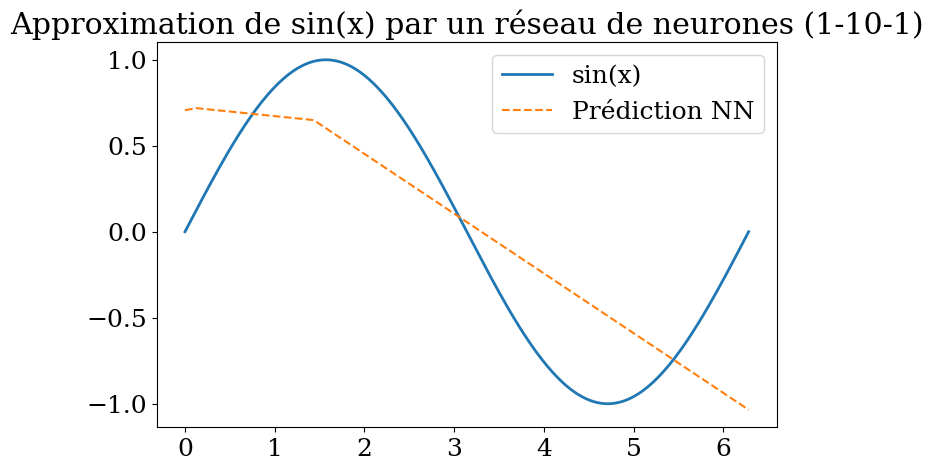
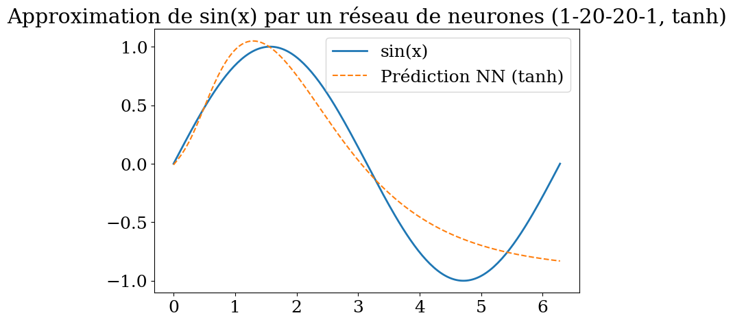
application to the prediction of sin(x) on \([0,2\pi]\) using a neural network 1-20-20-1
import numpy as np
import matplotlib.pyplot as plt

# Activation functions
def tanh(x):
    return np.tanh(x)

def tanh_deriv(x):
    return 1 - np.tanh(x)**2

# Mean Squared Error
def mse_loss(y_pred, y_true):
    return np.mean((y_pred - y_true) ** 2)

def mse_deriv(y_pred, y_true):
    return (y_pred - y_true) / y_true.shape[0]

# Réseau de neurones multi-couches avec tanh
class NeuralNetwork:
    def __init__(self, layer_sizes):
        """
        layer_sizes = [input_size, hidden1, hidden2, ..., output_size]
        """
        self.num_layers = len(layer_sizes) - 1
        self.W = []
        self.b = []

        for i in range(self.num_layers):
            in_size = layer_sizes[i]
            out_size = layer_sizes[i+1]
            # Xavier init
            self.W.append(np.random.randn(in_size, out_size) * np.sqrt(1. / in_size))
            self.b.append(np.zeros((1, out_size)))

    def forward(self, X):
        self.Z = []
        self.A = [X]

        for i in range(self.num_layers - 1):  # couches cachées
            z = self.A[-1] @ self.W[i] + self.b[i]
            a = tanh(z)
            self.Z.append(z)
            self.A.append(a)

        # Dernière couche (linéaire)
        z = self.A[-1] @ self.W[-1] + self.b[-1]
        self.Z.append(z)
        self.A.append(z)
        return z

    def backward(self, y_true, learning_rate=0.01):
        m = y_true.shape[0]
        dA = mse_deriv(self.A[-1], y_true)

        for i in reversed(range(self.num_layers)):
            dZ = dA
            if i < self.num_layers - 1:  # si ce n'est pas la sortie
                dZ = dA * tanh_deriv(self.Z[i])

            dW = self.A[i].T @ dZ
            db = np.sum(dZ, axis=0, keepdims=True)

            # Propagation en arrière
            dA = dZ @ self.W[i].T

            # Mise à jour
            self.W[i] -= learning_rate * dW
            self.b[i] -= learning_rate * db

    def train(self, X, y, epochs=5000, learning_rate=0.01):
        for epoch in range(epochs):
            y_pred = self.forward(X)
            loss = mse_loss(y_pred, y)
            self.backward(y, learning_rate)

            if epoch % 500 == 0:
                print(f"Epoch {epoch}, Loss: {loss:.6f}")

    def predict(self, X):
        return self.forward(X)
# ====== Expérience : approximation de sin(x) avec tanh ======
# Données
X = np.linspace(0, 2*np.pi, 200).reshape(-1, 1)
y = np.sin(X)

# Modèle : 1 entrée, deux couches cachées de 20 neurones tanh, 1 sortie
model = NeuralNetwork([1, 20, 20, 1])
model.train(X, y, epochs=5000, learning_rate=0.01)

# Prédictions
y_pred = model.predict(X)

# Visualisation
plt.figure(figsize=(8,5))
plt.plot(X, y, label="sin(x)", linewidth=2)
plt.plot(X, y_pred, label="Prédiction NN (tanh)", linestyle="--")
plt.legend()
plt.title("Approximation de sin(x) par un réseau de neurones (1-20-20-1, tanh)")
plt.show()
Epoch 0, Loss: 1.066883
Epoch 500, Loss: 0.115917
Epoch 1000, Loss: 0.089417
Epoch 1500, Loss: 0.081073
Epoch 2000, Loss: 0.076811
Epoch 2500, Loss: 0.073664
Epoch 3000, Loss: 0.071039
Epoch 3500, Loss: 0.068789
Epoch 4000, Loss: 0.066848
Epoch 4500, Loss: 0.065164
5.6.5. Type of Layers#
Dense Layer: Also known as a fully connected layer, this is a linear model where each neuron is connected to every neuron in the previous layer. It performs a matrix multiplication followed by an optional activation function to produce the output. This layer is used to learn linear relationships between features.
Convolutional Layer:
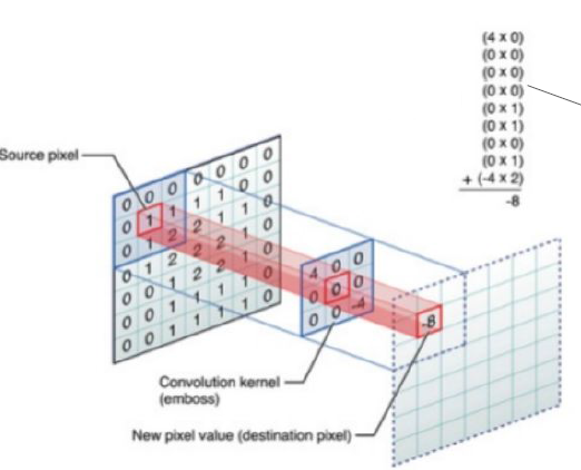
Purpose: Designed to handle spatial dimensions, such as images. This layer applies convolutional filters to local patches of the input to detect patterns like edges, textures, and shapes.
Hypothesis: Neighboring pixels represent similar information. By focusing on local regions, convolutional layers capture spatial hierarchies in the data.
Convolution Operation: Involves local connectivity of pixels (neighborhood) to detect larger objects such as lines and curves.
Max Pooling Layer:
Purpose: Reduces the spatial dimensions (width and height) of the input, typically after a convolutional layer. This layer performs a down-sampling operation by taking the maximum value from a specific region of the input.
Advantage: Helps to reduce the number of parameters and computations, and also helps to prevent overfitting by providing a form of translation invariance.
Dropout Layer:
Purpose: Regularization technique used to prevent overfitting. During training, randomly selected neurons are ignored (dropped out) with a certain probability.
Advantage: Helps the model generalize better by preventing reliance on any particular neurons.
Recurrent Layer:
Purpose: Designed to handle sequential or temporal data, such as time series or natural language. Recurrent layers maintain a hidden state across time steps, allowing the model to capture dependencies over time.
Types: Includes Long Short-Term Memory (LSTM) units and Gated Recurrent Units (GRUs), which are specifically designed to handle issues like vanishing and exploding gradients in long sequences.
5.6.6. Summary#
Dense Layer: Linear model connecting every neuron in the previous layer to every neuron in the current layer.
Convolutional Layer: Applies filters to local regions of the input, useful for detecting spatial patterns.
Max Pooling Layer: Reduces spatial dimensions by taking the maximum value from local regions, aiding in computational efficiency and overfitting prevention.
Dropout Layer: Regularization method that randomly drops neurons during training to improve generalization.
Recurrent Layer: Handles sequential data by maintaining a hidden state across time steps, capturing temporal dependencies.
These layers are fundamental components of various types of neural networks, including Convolutional Neural Networks (CNNs) for spatial data and Recurrent Neural Networks (RNNs) for temporal data.
5.7. Convolutional Neural Networks#
Convolution of an image
filter 5x5
5.7.1. Type of Convolutional Neural Networks#
objective: reduction of the data size (image)
\(\Rightarrow\) for an image, filter 3x3
Convolution
Max Pooling (replace several pixels by the max)
Drop Out (remove pixels)
5.7.2. Classification Neural network#
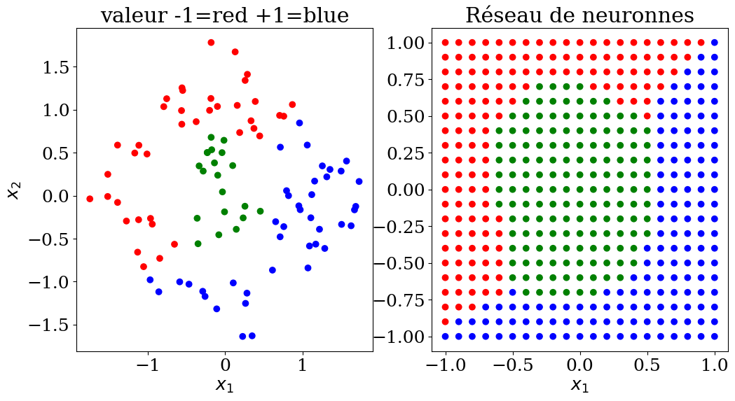
scikit learn model MLPClassifier
MLP = Multi-layer Perceptron
parameters:
hidden_layer_sizes = (taille1, taille2,…)
If you want a model with 3 layers, each containing 100 neurons, you should specify the model architecture as a tuple where each element represents the number of neurons in each layer. For this case, the tuple would be:
hidden_layer_sizes = (100,100,100).
The default value represents a single hidden layer of 100 neurons.
from sklearn.neural_network import MLPClassifier

N = 10
X,y,col = dataset3(N)
clf = MLPClassifier(hidden_layer_sizes=(N**2,N**2,N**2), max_iter=400, random_state=1, verbose = False)
clf = clf.fit(X,y)
print("score = {:2d}%".format(int(100*clf.score(X, y))))
score = 100%
# prediction
NN = 21
Xpred, ypred, colpred = predict3(NN, clf.predict)
plot3(X,col, Xpred,colpred,titre="Réseau de neuronnes")
5.7.3. Regression Neural network#
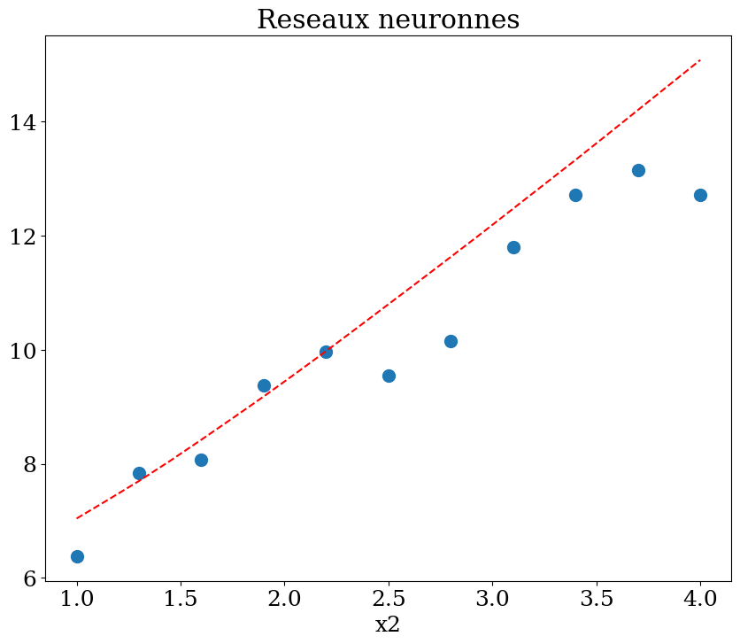
scikit learn model MLPRegressor
MLP = Multi-layer Perceptron
parameters:
hidden_layer_sizes = (number, size) 1,2, .. 5
from sklearn.neural_network import MLPRegressor

N = 11
X,y = dataset1(N)
clf = MLPRegressor(hidden_layer_sizes=(N**2,N**2,N**2), max_iter=400, random_state=1, verbose = False)
clf = clf.fit(X,y)
print("score = {:2d}%".format(int(100*clf.score(X, y))))
score = 43%
NN = 51
Xpred  = np.array([[1,x] for x in np.linspace(1,4,21) ])
ypred  = clf.predict(Xpred)
plot1(N,X,y, Xpred,ypred,titre="Reseaux neuronnes")
5.8. Learning with times series#
Classification
Identify rainy/non-rainy episodes
Determine if a weather station is malfunctioning
Regression
Predict the maximum temperature of the day
Predict the amount of expected rainfall
Correct the measured temperature
Problem
definition of the data \(X\) (features)
definition of the results \(y\) (target)
\(\Rightarrow\) machine learning: find the model \(f(X)\) that minimizes \(L\)
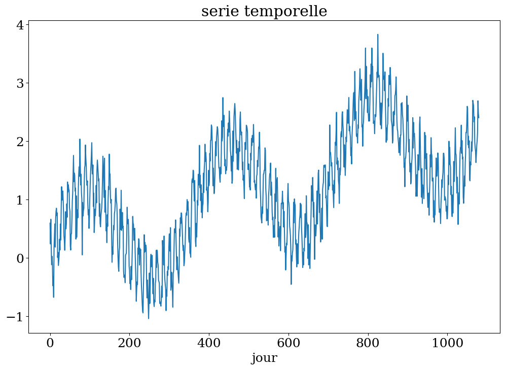
# construction serie
Ts,ys = serie_temp(3)
plt.figure(figsize=(12,8))
plt.plot(Ts[:],ys)
plt.xlabel("jour")
plt.title("serie temporelle");
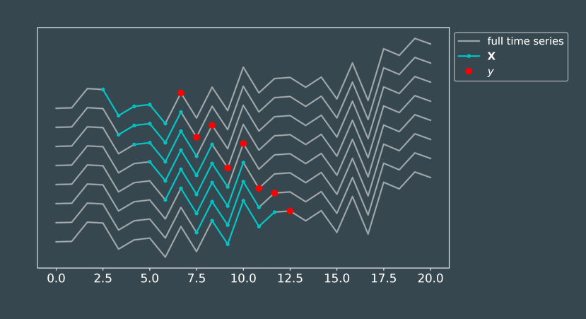
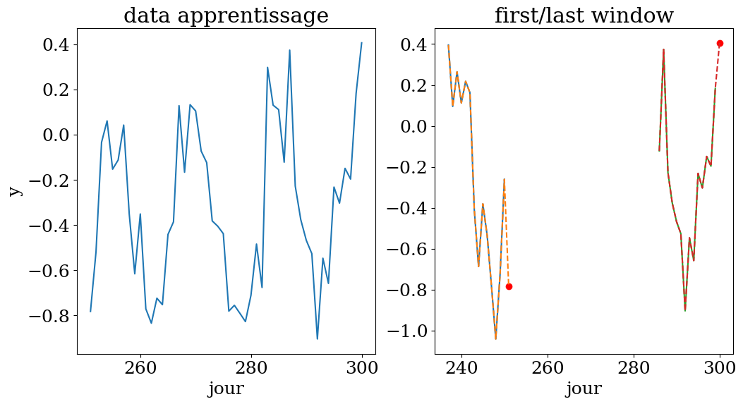
# 50 fenetres de 14 jours pour prediction au jour 300
n = 14
N = 50
t0 = 300
X,y,t = dataset4(Ts,ys,n,N,t0)
plot_data4(n,N,t0,t,X,y,Ts,ys)
apprentissage sur une fenetre de 14 jours entre le jour 237 et 300
from sklearn.linear_model import LinearRegression
from sklearn.ensemble import RandomForestRegressor
from sklearn.neighbors import KNeighborsRegressor
from sklearn.metrics   import r2_score
# choix de l'algorithme
clf = RandomForestRegressor()
#clf = KNeighborsRegressor()
#clf = LinearRegression()

clf.fit(X,y)
print("score = {:2d}%".format(int(100*clf.score(X, y))))
yp = clf.predict(X)
print("R2 = {:3.2f}%".format(r2_score(y,yp)))
score = 92%
R2 = 0.92%
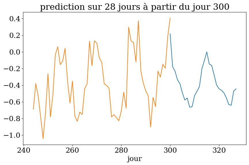
# prediction sur n1 jours
n1 = 2*n
Xpred  = np.zeros((n1,n))
ypred  = np.zeros(n1)
for k in range(n1):
    Xpred[k,:] = ys[t0+k-n:t0+k]
ypred = clf.predict(Xpred)
plot4(n1,t0,Ts,ys,ypred,"prediction")
5.9. Quality of Learning#
Regression Metrics to quantify the quality of predictions
For a test set (or training set) of size \(n\), the discrepancy between the prediction \(\hat{y}_i\) and the actual value \(y_i\) is evaluated.
Mean Squared Error (MSE):
The Mean Squared Error measures the average of the squares of the errors, which are the differences between the predicted values \(\hat{y}_i\) and the actual values \(y_i\). It is calculated as:
Where:
\(\hat{y}_i\) is the predicted value for the \(i\)-th observation.
\(y_i\) is the actual value for the \(i\)-th observation.
\(n\) is the number of observations in the test set.
MSE gives a measure of how well the model’s predictions match the actual values, with lower values indicating better performance.
Coefficient of Determination: \(R^2\) Score
It represents the proportion of the variance in \(y\) that has been explained by the independent variables of the model. It provides an indication of the quality of the fit and, consequently, a measure of how well unseen samples are likely to be predicted by the model, through the proportion of the explained variance.
The \(R^2\) score is calculated as:
Where:
\(\text{SS}_{\text{res}}\) is the sum of squared residuals (errors): \(\sum_{i=1}^{n} (\hat{y}_i - y_i)^2\)
\(\text{SS}_{\text{tot}}\) is the total sum of squares: \(\sum_{i=1}^{n} (y_i - \bar{y})^2\)
\(\bar{y}\) is the mean of the observed data \(y\)
An \(R^2\) score of 1 indicates a perfect fit, where all variance in the dependent variable \(y\) is explained by the model. An \(R^2\) score of 0 indicates that the model does not explain any of the variance in \(y\), and the model’s predictions are as good as the mean of the actual values.
5.10. Conclusion#
The choice of the right algorithm depends on:
The data: The nature, quality, and quantity of the data available can significantly impact which algorithm is most appropriate. For example, the presence of missing values, the distribution of the data, and the presence of temporal or spatial dependencies can all influence the choice.
Knowledge of the problem: Understanding the specific problem domain and the nature of the task (e.g., classification, regression, clustering) helps in selecting an algorithm that aligns with the problem’s requirements and constraints.
Choice of parameters: The performance of an algorithm can be heavily influenced by its hyper parameters. Choosing the right parameters (e.g., learning rate, number of layers, number of neighbors) through techniques like grid search or cross-validation can affect the effectiveness of the model.
5.11. References#
L’intelligence artificielle: introduction et applications en physique Bernet [2021]
Initiation au Machine learning en météo MétéoFrance [2018]
Apprentissage autosupervisé : IA, au tableau ! FranceCulture [2022]
from platform import python_version

print("Python version:",python_version())
print("numpy version:",np.__version__)
print("skitlearn version:",sk.__version__)
Python version: 3.10.12
numpy version: 1.26.4
skitlearn version: 1.1.3

