2. Minimization methods

Marc Buffat dpt mécanique, université Lyon 1

2.1. Introduction

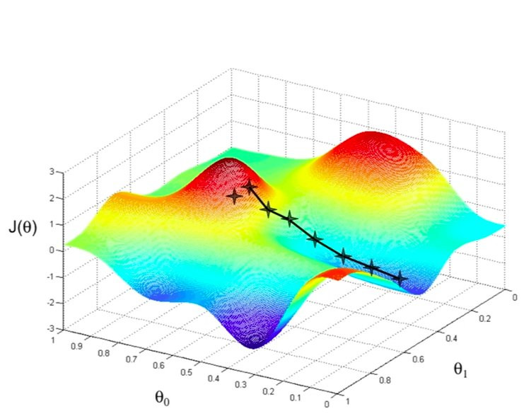
Example of an ill posed problem !!!

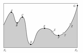
• There is no ideal method.

• It is easy to find a local minimum.

• It is difficult to find an absolute minimum.

Difficulties

• Importance of the initial guess (approximation)

• The minimization problem becomes much more difficult if the function depends on multiple variables

=> Minimizing in N dimensions for large N is very difficult

2.2. Minimization Algorithm (optimization)

To seek for the best prediction, we optimize (minimize) an objective function \(J\).

Optimization algorithms can be grouped into two categories : those that use derivatives and those that do not.

• Classical algorithms use the first derivatives (gradient) and sometimes the second derivatives (Hessian) of the objective function.

• Direct search and stochastic algorithms are designed for objective functions for which derivatives are not available.

Simple differentiable functions can be optimized analytically, such as the linear regression problem with 2 real parameters. Typically, the optimization of the objective functions, we are interested in, cannot be solved analytically.

Optimization is significantly easier if the gradient of the objective function can be calculated:

• \(\Rightarrow\) more efficient algorithms

2.2.1. Classical Minimization Algorithms

1. Bisection-type algorithm in 1D

2. Local descent-type algorithm in N dimensions

3. Non-local algorithm in N dimensions

Note: This taxonomy is inspired by the book “Algorithms for Optimization” Kochenderfer and Wheeler [2019]

2.3. Minimization Algorithms in 1D (bisection)

1D minimization (simple problem):

• only one parameter \(\beta\) such that \(F(\beta)\) is minimum

• exact solution if \(F(\alpha)\) is quadratic

\[F(\alpha)=a\alpha^2+b\alpha+c \mbox{ minimum for } \alpha_{opt} = -b/2a\]

• else use bisection type algorithm (ex Brent method \(\equiv\) quadratic interpolation + bi-section)

• equivalence between root finding and minimization

Bisection type algorithm

Bisection-type optimization algorithms are designed for optimization problems with a single input variable where the optima are known to exist within a specific range.

These algorithms are capable of efficiently navigating the known range and locating the optima, although they assume that only one optimum is present (the corresponding objective function is called unimodal objective functions).

Some algorithms can be used without information on derivatives if they are not available.

Examples of Bisection algorithms:

1. Basic bisection algorithm

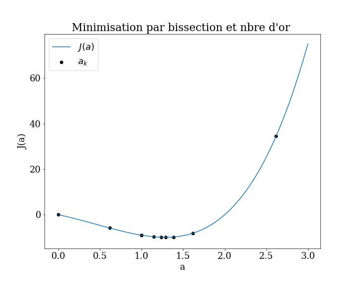
2. Golden search method (idem but instead of dividing by 2, we divide by the golden ratio \(\phi\))

3. Brent Optimization

in the scipy library: scipy.optimize

  scipy.optimize.minimize_scalar  
     method='brent', 'bounded', 'golden'
     
  Minimization of scalar function of one variable.

2.3.1. Root finding (\(\equiv\) minimization)

\[ \mbox{Find } a^* \mbox{ minimizing } F(a) \equiv J(a^*) = 0 \mbox{ with } J(a) = \frac{dF}{da}\]

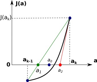
estimation of the root \(a^*\) \(J(a)\)

1. bisection method: milieu \(a^* \approx a_0 = \frac{a_{k}-a_{k-1}}{2}\)

2. secant method \(a^* \approx a_1 = a_{k} - J(a_k)\frac{a_k - a_{k-1}}{J(a_k) - J(a_{k-1}}\)

3. gradient method (Newton) \(a^* \approx a_2 = a_{k} - \frac{J(a_k)}{J'(a_k)}\)

Brendt: mix of the first two methods with a quadratic interpolation instead of a linear one

2.3.2. scipy.optimize.minimize_scalar

2.4. Local descent algorithm (dimension N)

Minimization in N dimension (complex problem for large N ):

• N parameters \(\mathbf{X}=\left[\beta_j\right]\)

One can reduce it to 1D minimization problems by choosing descent directions \(\mathbf{p_k}\)

• to minimize \(F(\mathbf{X})\) with \(X\in \mathcal{R}^N\)

Algorithm

• repeat

  1. choose a direction \(\mathbf{p}_k\) (p.e. \(-\nabla \mathbf{X}\))

  2. 1D minimization in the direction \(\mathbf{p}_k\)

  \[ \mbox{Find $\alpha$ that minimizes } F(\mathbf{X}_k + \alpha \mathbf{p}_k) \]

  4. new solution \(\mathbf{X}_{k+1}\)

  \[ \mathbf{X}_{k+1} = \mathbf{X}_k + \alpha_{opt} \mathbf{p}_k \]

Local descent optimization algorithms are designed for optimization problems with more than one input variable and a single global optimum (for example, with an unimodal objective function).

The most common example of a local descent algorithm is the line search algorithm:

• Line Search: $\(\mathbf{x}_{k+1}=\mathbf{x}_{k}+\alpha _{k}\mathbf {p} _{k}\)$

Here, \(x_k\) is the current point, \(p_k\) is the search direction, and \(α_k\) is the step size.

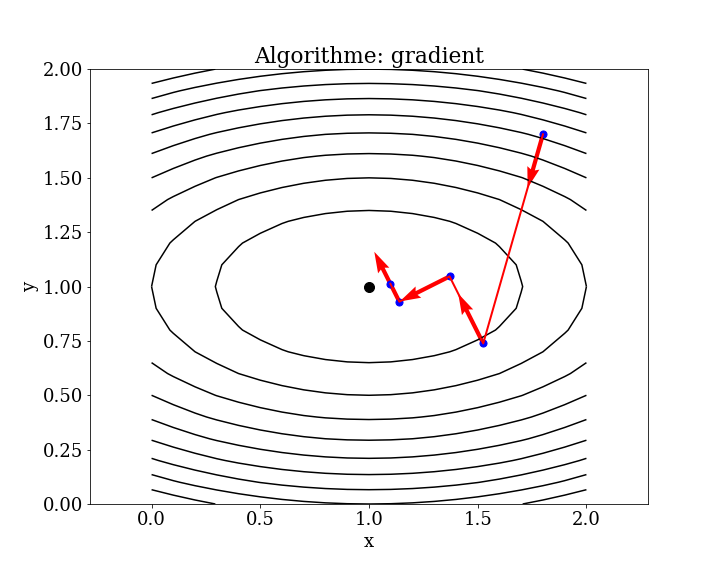
• Local Gradient Descent: In this case,

  \[ \mathbf{p}_k = -\vec{\nabla} J\]

where \(\vec{\nabla} J\) is the gradient of the objective function \(J\). The direction of descent is the negative gradient, and the step size \(\alpha_k\) is determined by the line search.

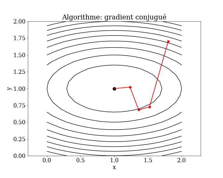
• Conjugate Gradient Method: This method improves upon gradient descent by using conjugate directions rather than simple negative gradients. It aims to accelerate convergence by ensuring that each search direction is conjugate (orthogonal) to the previous directions.

2.4.1. Line search

There are many variants of this algorithm (for example, the Brent-Dekker algorithm), but the procedure generally involves choosing a direction to move in the search space and then performing a bisection-type search along a line or hyperplane in the chosen direction.

Line search Algorithm

1. Step \(k\):

2. Compute a descent direction \(\mathbf{p}_k\)

3. Choose \(\alpha_k\) as the value that minimizes the 1D function \(\phi(\alpha)\)

\[\phi (\alpha )=f(\mathbf{x} _{k}+\alpha \mathbf{p} _{k})\]

4. Update \(x_k\)

\[\mathbf{x}_{k+1}=\mathbf{x}_{k}+\alpha _{k}\mathbf {p} _{k}\]

5. Iterate if the desired accuracy is not reached.

Remarks

This process is repeated until no further improvement can be achieved.

The limitation is that it is computationally expensive to optimize each directional move in the search space.

In scipy.optimize, the generic function minimize is used to perform optimization tasks. This function can handle a variety of optimization problems, including those involving local descent algorithms and other optimization methods. It provides a unified interface for different optimization algorithms and is designed to handle various kinds of objective functions and constraints.

2.4.2. line_search (scipy.optimize.line_search)

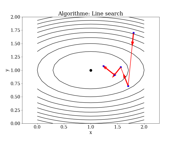
2.4.2.1. local gradient method (GM)

2.4.3. conjugate gradient method (CG)

2.5. First order algorithms (generalization)

First-order optimization algorithms explicitly use the first derivative (gradient) to determine the direction to follow in the search space.

The procedures generally involve the calculation of the gradient of the function and then following the gradient in the opposite direction (e.g., moving towards the minimum for minimization problems) using a step size (also known as the learning rate in AI).

The step size is an hyper parameter that controls the distance to move in the search space, in contrast to local descent algorithms, which perform a full line search for each directional move

Remarques

A step size that is too small results in a search that is time-consuming and may get stuck, while a step size that is too large can cause zigzags or oscillations in the search space, potentially missing the optima entirely.

First-order algorithms are generally referred to as gradient descent methods, with more specific names denoting minor extensions of the basic procedure.

2.5.1. Descent algorithm using stochastic gradient (SGD)

The gradient descent algorithm also provides the model for the popular stochastic version of the algorithm, called Stochastic Gradient Descent (SGD), which is used to train artificial neural network models (deep learning).

The key difference is that the gradient is approximated rather than computed directly, using prediction errors on training data, such as a single sample (stochastic), all examples (batch), or a small subset of training data (mini-batch).

Extensions designed to accelerate the gradient descent algorithm (momentum, etc.) can and are commonly used with SGD and AI.

2.5.2. Stochastic gradient method (full batch)

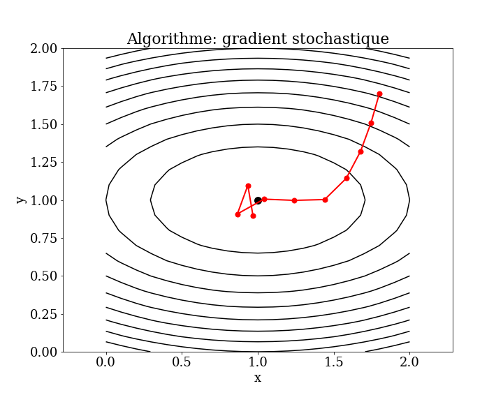
2.5.3. Stochastic Gradient Descent

At each step of the gradient descent, instead of using the entire dataset (e.g., for a smoothing problem), the algorithm can use a subset of the data. This approach involves approximating the gradient based on a smaller portion of the data rather than the whole dataset.

Minimization of the Objective Function in n dimension: \(J(\mathbf{w}=\{w_k\}_{k=1,n})\)

gradient method

\[ \mathbf{w} = \mathbf{w} - \alpha \nabla J(\mathbf{w}) = \mathbf{w} - \frac{\alpha}{n} \sum_{i=1}^n \nabla J_i(\mathbf{w})\]

stochastic gradient

In Stochastic Gradient Descent (SGD), instead of using the entire dataset, the algorithm iterates over the data one sample at a time:

\[ \mathbf{w} = \mathbf{w} - \alpha \nabla J_i(\mathbf{w})\]

The step size is denoted by \(\alpha\) (called the learning rate in machine learning)

2.5.4. Mini-batch

• Full Batch Gradient Descent: The gradient is computed over the entire data set.

  Disadvantage: Too slow for a large data set.

• SGD (Stochastic Gradient Descent): The gradient is estimated sample by sample.

  Disadvantage: Slow and has more chaotic convergence.

• Mini-Batch Gradient Descent: Compromise

  The gradient is estimated over \(k\) samples at a time (e.g., 32 samples).

This is the method used in practice

2.5.5. Epoch

In SGD (Stochastic Gradient Descent), the gradient is estimated either sample by sample or by mini-batches of a few samples.

• A complete pass over the dataset is called an Epoch.

• The number of epochs refers to the number of passes made over the training data set during the learning process.

2.6. Non-Differentiable Objective Functions

Optimization algorithms that use the derivative of the objective function are generally fast and efficient.

But challenges for Objective Functions due to :

1. Complexity of the Function: Some objective functions are so complex that computing their derivatives is impractical. For instance, functions involving high-dimensional data or intricate interactions between variables may be difficult to differentiate.

2. Non-Differentiability: In certain cases, the function may not be differentiable everywhere. Functions with discontinuities, sharp corners, or non-smooth regions pose challenges for gradient-based methods.

3. Derivative Information Not Useful: Even if derivatives can be computed, they may not always provide useful guidance. For example, the gradient may be very small or oscillatory, leading to slow convergence or poor directionality.

Consequently, these challenges make it difficult to apply traditional gradient-based algorithms effectively for such objective functions.

difficulties

When dealing with certain types of objective functions, traditional gradient-based optimization algorithms may not be suitable. Some common challenges include:

• No Analytical Description of the Function: For example, in simulations where the function is defined by complex processes rather than explicit equations.

• Multiple Global Optima: For example, in multimodal functions where multiple peaks or valleys exist.

• Stochastic Evaluation of the Function: For example, when the function evaluation is noisy or involves random fluctuations.

• Discontinuous Objective Function: For example, when the function has abrupt changes or regions with invalid solutions.

Given these challenges, there are optimization algorithms that do not rely on first-order or second-order derivatives

classification of these algorithms

These algorithms are sometimes referred to as black-box optimization algorithms because they make few or no assumptions about the objective function, unlike classical methods.

These algorithms can be classified into:

1. Direct Algorithms (Local):

   • These algorithms perform a systematic search in the local neighborhood of the current solution. They are designed to explore the immediate vicinity to find a better solution.

   • Example: Nelder-Mead method (Downhill Simplex), which does not use gradient information and explores the local region by reflecting, expanding, contracting, and shrinking the simplex.

2. Stochastic Algorithms (Non-Local):

   • These algorithms incorporate randomness in the search process to explore the search space more broadly and are capable of escaping local optima to find global solutions.

   • Example: Simulated Annealing, which uses random sampling and probabilistic decisions to explore the search space, allowing uphill moves to escape local minima.

3. Genetic Algorithms (Non-Local):

   • These algorithms are inspired by the process of natural selection and use mechanisms such as selection, crossover, and mutation to evolve a population of candidate solutions over generations.

   • Example: Genetic Algorithms (GA), which operate on a population of solutions and use genetic operators to explore the search space and find global optima.

2.6.1. Directs Algorithms

Direct optimization algorithms are designed for objective functions where derivatives cannot be calculated. These algorithms are deterministic procedures and often assume that the objective function has a single global optimum, such as in unimodal functions.

Direct search methods are also generally referred to as “pattern search” because they navigate the search space using geometric shapes or decisions, e.g., patterns.

Gradient information is approximated directly (hence the name) from the objective function’s result by comparing the relative difference between scores for points in the search space. These direct estimates are then used to choose a direction to move in the search space and triangulate the region of the optima.

Key Characteristics of Direct Optimization Algorithms:

• Gradient-Free: These methods do not require gradient information, making them suitable for non-differentiable or noisy objective functions.

• Deterministic Nature: They follow a deterministic process, meaning that given the same starting point and settings, they will always produce the same result.

• Pattern Search: The algorithms use predefined patterns or shapes to explore the search space. Common strategies include evaluating points on a grid or along specific directions.

• Triangulation of Optima: By comparing objective function values at different points, these methods estimate gradients and use this information to triangulate the search region, progressively honing in on the optimum.

Examples of directs algorithms :

• Powell Method

  Searches along a set of conjugate directions, updating the directions based on previous search results to find the optimum without gradient information.

• Hooke-Jeeves Method

  Alternates between exploratory moves (searching along coordinate directions) and pattern moves (combining directions) to find improvements

• Simplex Method: Nelder-Mead

  Uses a simplex (a polytope of n+1n+1 vertices in nn-dimensional space) to explore the search space and adjust its size and shape based on function evaluations.

By using these methods, direct optimization algorithms can effectively handle complex, non-smooth, and noisy objective functions, providing robust solutions where classical gradient-based methods may fail

2.6.1.1. Nelder-Mead Simplex Method

simplex: generalization of the notion of triangle or tetrahedron to arbitrary dimensions. A n-simplex is a n-dimensional polytope that is the convex hull of its n + 1 vertices in \(\mathcal{R}^n\)

Starting initially from such a simplex, it undergoes simple transformations during the iterations: it deforms, moves, and progressively shrinks until its vertices converge to a point where the function is locally minimal.

Principle in 2D

• Start with 3 points forming a triangle, determine the point where the function is at its maximum, and calculate the reflection point relative to the other two.

• If the value at this new point is lower than all the others, construct a simplex with this point and return to step 1.

• If the value is better than the second but worse than the best, replace the second point and return to step 1.

• If the value is higher than all the points, the minimum is within the initial simplex. Contract this simplex and return to step 1.

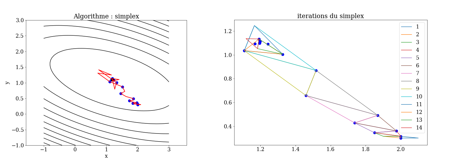
Nelder-Mead Simplex Method Process

• Initialization:

  Start with an initial simplex consisting of \(n+1\) vertices in a n-dimensional space.

• Iteration / transformation

  The simplex continually deforms and moves through the search space as it adapts to the landscape of the objective function.

  • Reflection: Reflect the worst vertex through the centroid of the remaining vertices to explore a potentially better point.

  • Expansion: If the reflection point is better than the best vertex, expand further in this direction to see if an even better point can be found.

  • Contraction: If the reflection point is not better than the second-worst point, contract the simplex towards the better points to focus the search.

  • Shrinkage: If the contraction does not yield a better point, shrink the entire simplex towards the best vertex, reducing its size.

• Convergence:

  The simplex gradually shrinks and its vertices get closer, zeroing in on a local minimum. The process continues until the vertices are sufficiently close to each other, indicating that the function has been minimized locally.

By iterating through these steps, the simplex adjusts its shape and size, effectively navigating the search space to find a local minimum. This method is robust for many types of optimization problems, particularly those where derivative information is not available.

2.6.1.2. Powel Algorithm

The method minimizes the function by a bidirectional line search. The line search method along each search vector can be performed using a golden section search or the Brent’s method.

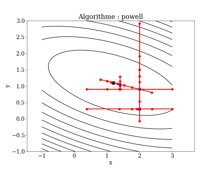
Powell’s Algorithm

The method minimizes the function using a bidirectional line search technique. The line search along each search vector can be performed using either the golden section search or Brent’s method.

Successive descent directions are chosen along each coordinate (parameter), and minimization is performed in 1D along this direction.

\[\{x_{0}+\alpha_{1}s_{1},{x}_{0}+\sum_{i=1}^{2}\alpha_{i}{s}_{i},\dots ,{x}_{0}+\sum_{i=1}^{N}\alpha_{i}{s}_{i}\}\]

and we choose:

\[x_1 = {x}_{0}+\sum_{i=1}^{N}\alpha_{i}{s}_{i}\]

then we iterate.

The method is useful for calculating the local minimum of a continuous but complex function, especially one without an underlying mathematical definition, because it does not require taking derivatives. The basic algorithm is simple; the complexity lies in the line searches along the search vectors, which can be performed using Brent’s method.

2.6.2. Stochastic Algorithms

A meta heuristic is an optimization algorithm designed to solve difficult optimization problems for which no more efficient classical method is known.

Meta heuristics are generally iterative stochastic algorithms that progress towards a global optimum (i.e., the global extremum of a function) by sampling an objective function.

Stochastic optimization algorithms are methods that incorporate randomness in the search procedure for objective functions where derivatives cannot be calculated. Unlike deterministic direct search methods, stochastic algorithms typically involve much more extensive sampling of the objective function, but they are capable of handling deceptive local optima.

Key Characteristics of Stochastic Optimization Algorithms

• Random Sampling: These algorithms use random sampling to explore the search space, making them suitable for complex and noisy objective functions.

• Escape Local Optima: By incorporating randomness, these methods can escape local optima and have a better chance of finding the global optimum.

• Extensive Exploration: They often perform extensive exploration of the search space, which can lead to better solutions for difficult optimization problems.

Main Algorithms

• Simulated annealing

• Evolution strategy

2.6.2.1. Simulated annealing

Simulated annealing is an empirical (metaheuristic) optimization method inspired by a process used in metallurgy. The algorithm alternates cycles of slow cooling and reheating (annealing) to minimize the energy of a material. The most stable configuration is reached by controlling the cooling process and slowing it down by adding heat.

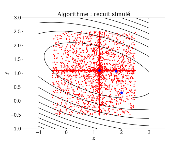
Simulated Annealing Algorithm

Inspired by Metallurgy: The algorithm is inspired by the annealing process in metallurgy, where a material is heated and then slowly cooled to remove defects and find a state of minimum energy.

Process:

• Initialization: Start with an initial solution and a high temperature. -Iteration:

  • Generate a new solution by making a small random change to the current solution.

  • Calculate the change in the objective function (\(\Delta J\)).

  • If the new solution is better (\(\Delta J<0\)), accept it.

  • If the new solution is worse (\(\Delta J>0\)), accept it with a probability that decreases with temperature.

Cooling Schedule: Gradually reduce the temperature according to a cooling schedule.

Convergence: The process continues until the system “freezes” and no further improvements can be made.

Algorithm:

• Start with \(N\) randomly chosen points and a high temperature \(T\).

• Evolution at constant \(T\):

  1. Calculate the energy \(E\) (error) at each point.

  2. Randomly perturb the points (positions), causing their energy to change by \(\Delta E\)

  3. If \(\Delta E < 0\), accept the new position; otherwise, accept it with probability \(e^{-\Delta E/T}\)

  4. Iterate step 3 until there is little change (thermodynamic equilibrium at \(T\)).

• Decrease the temperature \(T\) and repeat from second step

2.6.2.2. Evolution strategy algorithm

Inspired by Natural Evolution: Evolution strategies (ES) are inspired by the process of natural selection and evolution.

Process:

• Initialization: Start with an initial population of candidate solutions.

• Evaluation: Evaluate the fitness of each candidate solution based on the objective function.

• Selection: Select the best-performing solutions to act as parents.

• Reproduction: Generate a new population through recombination and mutation of the parents.

• Iteration: Repeat the evaluation, selection, and reproduction steps for a number of generations.

• Convergence: The process continues until a satisfactory solution is found or a predetermined number of generations is reached.

Main algorithms

• genetic algorithm

• differential evolution algorithm

2.6.2.3. differential evolution

The differential evolution algorithm is a stochastic meta-heuristic optimization method inspired by genetic algorithms and evolution strategies, combined with a geometric search technique. While genetic algorithms modify the structure of individuals using mutation and crossover, evolution strategies achieve self-adaptation through geometric manipulation of individuals.

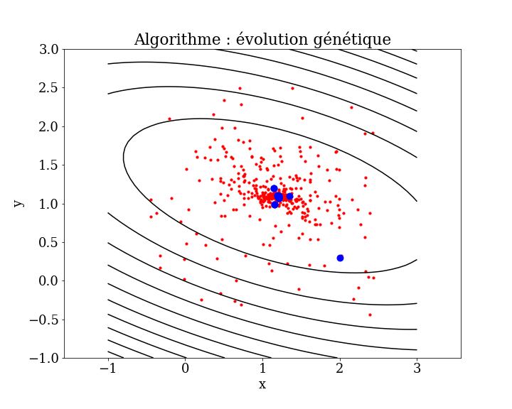
Key Concepts of differential evolution algorithm

• Population-Based Approach:

  Differential evolution works with a population of candidate solutions, evolving them over generations to find the global optimum.

• Initialization:

  The algorithm starts with a randomly initialized population of potential solutions within the search space.

• Mutation:

  Mutation is performed by adding the weighted difference between two population vectors to a third vector, creating a mutant vector.

• Crossover:

  Crossover combines the mutant vector with a target vector to create a trial vector. This is typically done using binomial (uniform) or exponential crossover methods.

• Selection:

  Selection is done by comparing the trial vector to the target vector. The one with the better objective function value is selected for the next generation.

• Geometric Manipulation:

  Evolution strategies use geometric manipulation to adapt and evolve the population. This involves the spatial arrangement and geometric relationships between vectors.

• Self-Adaptation:

  Differential evolution allows the algorithm parameters, such as the scaling factor and crossover rate, to adapt dynamically based on the search process.

Differential evolution effectively combines aspects of genetic algorithms and evolution strategies with a focus on geometric transformations. This combination allows it to perform robust searches across complex, multimodal landscapes, making it well-suited for various optimization problems. The algorithm’s reliance on population-based search and self-adaptation helps it navigate and exploit the search space efficiently, overcoming challenges such as local optima and non-differentiable objective functions.

2.7. Conclusion

Tackling a Minimization Problem

Objective: Minimize the function \(F(x_1, ..., x_n)\) with \(N\) variables.

First question: Is the Problem Well-Posed (Simple)?

• Criteria:

  • Idea of a minimum: The function has a clear and identifiable minimum.

  • Absence of numerous parasitic minima: The function does not have many local minima that can mislead the optimization process.

• Decision:

  • If Yes: The problem is simple and well-posed.

    Use Deterministic Methods: These methods leverage the derivatives of the function for efficient and precise optimization.

    Examples: Gradient descent, Newton’s method, Conjugate gradient method.

  • If No: The problem is complex and not well-posed.

    Use Stochastic Methods: These methods incorporate randomness to explore the search space and are robust against deceptive local optima.

    Examples: Simulated annealing, Differential evolution, Genetic algorithms.

Practical Approach

• Assess the Problem: Determine whether the problem is well-posed or complex based on the criteria above.

• Select the Appropriate Method:

  • Deterministic Methods: For well-posed problems with clear minima and smooth objective functions.

  • Stochastic Methods: For complex problems with many local minima, non-differentiable or noisy objective functions, and discontinuities.

By following this structured approach, you can choose the most effective optimization method tailored to the characteristics of your specific minimization problem.

2.8. Reference

1. Convex Optimization Boyd and Vandenberghe [2004]

2. Computational Intelligence: An Introduction (Second Edition) Engelbrecht [2007]

3. Algorithms for Optimization Kochenderfer and Wheeler [2019]

4. Algorithmes de minimisation (master course) Charnoz and Daerr [2010]

5. Optimisation (mathématiques) wikipedia [2024]