3.6. Introduction to AI/ML#
Marc Buffat dpt mécanique, université Lyon 1
AI = Artificial Intelligence, ML = Machine Learning
inspired by Cardon, Cointet, and Mazières [2018] and MétéoFrance [2018]

%%html
<style>
td,th {font-size: 24px}
</style>
3.6.1. Artificial Intelligence#
Artificial intelligence is undoubtedly one of the major challenges of modern science. It refers to the theories and models that enable the creation of machines capable of autonomously simulating human intelligence. Within the concept of artificial intelligence, there are commonly distinguished fields such as deep learning and machine learning. While machine learning encompasses systems that learn from large datasets, deep learning consists of systems that learn through neural networks made up of algorithms capable of functioning without structured data and entirely autonomously without human intervention.

Today, Artificial Intelligence is present in almost every aspect of daily life, from our smartphones to our cars, and this technology is attracting an increasing number of companies such as Amazon, Google, Microsoft, and Facebook
3.6.1.1. Definition of ARTIFICIAL INTELLIGENCE (an attempt!)#
Definition of AI : (Kurzweil, 1990)
The art of creating machines with capabilities that require intelligence when performed by humans
Moravec’s Paradox : (years 80)
it is comparatively easy to make computers exhibit adult level performance on intelligence tests or playing checkers, and difficult or impossible to give them the skills of a one-year-old when it comes to perception and mobility
3.6.1.2. Historical view:#
The four ages of Artificial Intelligence Cardon, Cointet, and Mazières [2018]
Computer/Software |
World |
Method |
Horizon |
|---|---|---|---|
Cybernetic (data connection) |
Environment |
« Black Box» |
Negative feedback |
Symbolic AI (symbolic) |
Toy world |
Logical |
Resolution of problem |
Expert System (symbolic) |
Expert knowledge |
Hypothesis selection |
Examples/ counter-examples |
Deep Learning (data connection) |
The world is a vector of BIG DATA |
Deep neural network |
Minimization of the error on the objective function |
3.6.1.3. Questions ?#
Will Wilson : nov. 2017
“What’s the difference bewteen AI and ML ?”
It’s AI when you’re raising money,
it’s ML when you’re trying to hire people.
3.6.2. Learning method in AI (machine learning)#
Supervised learning (the most commonly used)
but needs huge training data-base
Reinforcement learning (chess, GO)
focus on finding a balance between exploration (of uncharted territory) and exploitation (of current knowledge) with the goal of maximizing the long term reward, whose feedback might be incomplete or delayed (WIKIPEDIA)
Unsupervised learning
model that tries to find any similarities, differences, patterns, and structure in data by itself
generative task (language, translation, ..)
LLM (Large Language Model)
The scientific method: France Culture FranceCulture [2022]
Attention: importance of the learning data set
Researchers in AI at Cambridge have demonstrated that AI models can degrade in accuracy and effectiveness if they are repeatedly trained on their own generated outputs.
3.6.3. Classical examples#
AI for handwriting recognition

AI for facial recognition
SPAM detection/ social network
3.6.4. AI application in Mechanical Engineering#
3.6.4.1. Machine Learning#
data processing
structured data
supervised learning
3.6.4.2. Deep Learning#
use of large neural networks (LNN)
Big Data
3.6.4.3. Prediction of the mechanical properties of steels#
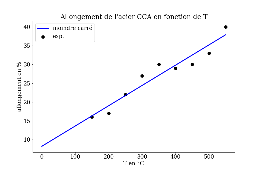
Based on an experimental data set for different steel alloys, prediction of the material’s properties (elongation) as a function of its composition and temperature.
3.6.4.4. Prediction of the hydrodynamic properties of pleasure boats#
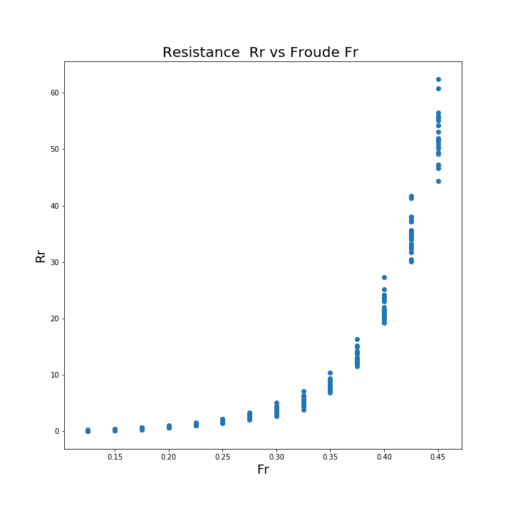
Prediction of the hydrodynamic properties (\(R_r\) resistance to advancement: wave + friction) based on geometric characteristics and speed: Froude \(Fr=\frac{U}{\sqrt{gL}}\)
3.6.4.5. Machine Learning from Numerical Simulation (FEM)#
Engineers use numerical models to analyze the behavior of systems for parametric studies. This provides great flexibility to modify parameters and find the best design.
However, when models are too complex, numerical simulations can easily take a very long time: from several hours to several days. Additionally, during the optimization process, you might need to run dozens of trials. To simplify the process, we can build a simpler model based on a few simulations using machine learning.
3.6.4.6. Meteorologic prediction using AI#
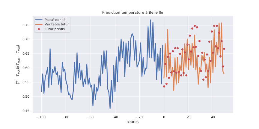
Currently, weather forecasting programs are based on physical models. However, these physical models are computationally expensive. Companies like Google have already produced work demonstrating remarkable speedups compared to state-of-the-art physical methods by designing machine learning-based neural networks to predict local weather
3.6.4.7. Physics-Informed Neural Networks (PINN)#
This new class of neural networks hybridizes machine learning with physical laws, allowing for “better” predictions from neural networks (Deep Learning) for physical applications governed by equations (ODEs or PDEs): see Hairy [2022]
Physics-informed neural networks !!!
Note: These neural networks only account for constraints related to the physical properties of the studied system
there is no actual understanding of physics in these algorithms.
from IPython.display import YouTubeVideo
print("Application in Fluid Mechanics by S. Brenton , University of Washington")
YouTubeVideo('8e3OT2K99Kw', width=800, height=400)
Application in Fluid Mechanics by S. Brenton , University of Washington
3.6.4.7.1. Discrepancy models#
idealized systems
idealized Hamiltonian or Lagrangian system
knowledge of constraints, conservation laws, symmetries
real systems
discrepancy terms: \(\delta g (\mathbf{x})\)
model \(\delta g (\mathbf{x})\) using ML (PINNS)
reference:
from IPython.display import YouTubeVideo
print(" Discrepancy Modeling with Physics Informed Machine Learning by S. Brenton , University of Washington")
YouTubeVideo('7n7xaviepKM', width=800, height=400)
Discrepancy Modeling with Physics Informed Machine Learning by S. Brenton , University of Washington
remarks: it is important to understand how this idea has historically manifested itself and what engineers can learn about when to apply machine learning to model dynamical systems and what potential issues may arise.
On the following video, the difference between the Earth-centric solar system and the sun-centric solar system is illustrated.
Prior to this understanding, the dynamics were thought to be extremely complicated when the Earth was believed to be at the center of the solar system. It is difficult to find a simplistic, ideal model to describe this behavior. However, it is much easier to create a simple model when the appropriate coordinate system is used (Newton law).
What is important to note here is that it took a considerable amount of time to shift from the Aristotelian model and Ptolemy’s circular system centered on earth, to Kepler’s laws of motion in the sun-centric Copernican system. Interestingly enough, the Ptolemy system, which was in the incorrect coordinate system and had the wrong physics, was more accurate for a prolonged period than Kepler’s model, which had the correct physics and placed the sun at the center of the solar system.
from IPython.display import YouTubeVideo
print("Heliocentrism and Geocentrism by David Velasco")
YouTubeVideo('ZeS8h1t-uMA', width=800, height=400)
Heliocentrism and Geocentrism by David Velasco
3.6.5. Tools for AI#
basic libraries available in Python
numpy, scipy : numerical method
pandas : data base
seaborn: statistical data visualization
3.6.5.1. scikit-learn: Machine Learning in Python (open source)#
simple and effective tools for data analysis
based on NumPy, SciPy and matplotlib
import sklearn
3.6.5.2. tensor-flow: (open source)#
Machine learning libraries developed by Google
Keras: a high-level API for TensorFlow in Python
Optimization (multi-processing / GPU)
import tensorflow
3.6.5.3. torch / Pytorch (open source)#
PyTorch: AI libraries developed by META (Facebook)
import pytorch
3.6.6. Challenges in Machine Learning#
Goal : prediction of a function \(\mathcal{F}\)
using Machine Learning from a training data base \(\textbf{X}_i, Y_i\)
\(\rightarrow\) Minimization Problem
Find the best approximation \(\mathbf{F}\) that minimizes the error \(J\) on training data-base. \(J\) is a cost function such as:
Evaluate the approximation on a test data-base.
3.6.7. Modeling of experimental data#
3.6.7.1. Study of the dilatation of a metallic bar#
measure of the length as a function of the temperature
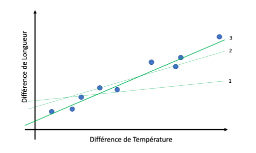
Modeling involves fitting a curve to data to make predictions.
The simplest model is a linear fit, which can be determined mathematically using the least squares method that minimizes the quadratic error between the measurement points and the model.
The model is simple and has only 2 parameters. From the model, predictions can then be made.
Machine learning is exactly that: fitting a model to data!
3.6.7.2. Artificial Intelligence Revolution#
Compared to our previous example, it’s just a matter of scale.
First, the most advanced models today, especially in the field of language processing, can have more than 100 billion parameters, while our thermal expansion model has only two.
Second, these models require a phenomenal amount of data, often collected automatically from millions or even billions of web pages. In the example above, we trained our model with only 9 data points.
Finally, these models can work with very high-dimensional data (Big Data).
In the thermal expansion example, we considered two-dimensional data: each point is represented by two variables, the change in length and the change in temperature.
In contrast, a neural network for image classification works with images made up of pixels, with each pixel having three color levels (red, green, blue) ranging from 0 to 255. Thus, a 200x200 pixel image can be considered a “point” in a 200x200x3 = 120 000 dimensional space!
This has been made possible by two technological advancements:
Hardware: the increase in computing power (multi-core and GPUs)
Software: and the Internet (data collection -> machine learning)
3.6.8. Introduction to Machine Learning#
problem: find the vector state Y from an observed state (data) X, i.e. the function $\( Y = F(X) \)$
the function \(F(X)\) is not known analytically
\(\Rightarrow\) it must be defined “optimally”:
Necessity of a training database (learning database)
Necessity of a validation (test database)
remarks
No “real intelligence”, but search for correlations (through non-linear processes)!
No explanatory power!
Importance of the quality of the database and the choice of inputs X
Need of a (critical) analysis of the result
3.6.8.1. Major categories of machine learning algorithms#
different types of machine learning
Supervised Learning |
Unsupervised Learning |
|---|---|
The training data is labeled |
The data is provided |
with the expected results. |
without the expected output labels |
3.6.8.2. Classification / Regression#
Regression |
Classification |
|---|---|
Prediction of a quantitative variable |
Prediction of a class membership (qualititive, discrete) |
3.6.9. A first method in Machine Learning : the linear regression#
goal: predict the elongation of steel as a function of temperature
Supervised Machine Learning :
A training data-set X, y obtained from measurements
X : is the temperature in °C (observable / data)
y : is the elongation in % (prediction / target)
3.6.9.1. Find the straight line that best fits the scatter of experimental points#

best solution = linear regression
3.6.10. Linear regression and cost function#
Let \(\{X_i,y_i\}_{i=1,m}\) be a sample of size m from the training data-set
3.6.10.1. How to define the best prediction \(h(x)\) ?#
In this simple case, we can define the prediction \(h(x)\) explicitly as a function depending on 2 parameters \(a\) and \(b\):
The “best” prediction \(h(x)\) (straight line) is the one that minimizes a cost function \(J\) that measures the mean squared error between the prediction and the actual value for the sample.
3.6.10.2. Cost Function \(J(a,b)\)#
example : quadratic error
\(\leadsto\) Minimization Problem
remarks
For this simple problem, an analytical solution exists (Least squares line)
solution of the linear system: \(\nabla J(a,b)=0\)
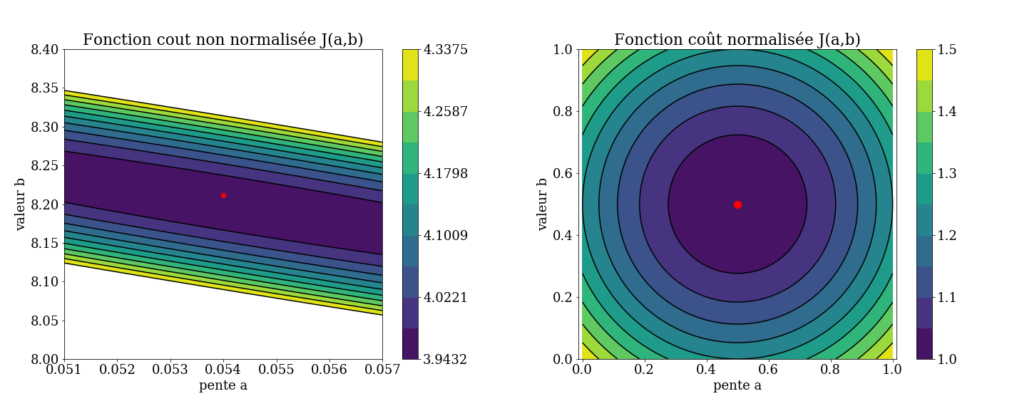
Importance of the normalization
\(\leadsto\) form of the cost function
Difficulty of the minimization probleme
form of the cost functions \(J(a,b)\)
3.6.11. Conclusion#
Machine learning: prediction of the value of a function (value of \(y\)) from the data (observable) \(X\)
\(F(X)\) non linear transformation of the data \(X\) (observable) to get a prediction (state vector) \(y\)
Questions
choice of the transformation \(h(x)\) and the parameters \(a_i\)
data processing
based on assumed correlations between the results and the data
is it intelligence?
No, it is not intelligence. What you’re describing involves finding correlations between results and data, which is a mathematical and statistical process. It does not imply actual understanding or cognition.
Intelligence generally involves reasoning, learning, and adapting in a way that mimics human cognitive abilities. The process of finding correlations or fitting models to data is a tool used within the broader scope of artificial intelligence, but by itself, it does not constitute intelligence.
3.6.11.1. Methodology#
Learning phase (training)
Definition of the best parameters \(a_i\) that allow for the prediction of the optimal value on a training data-set \(X^k,y^k\)
Minimization problem of a cost function \(J\)
Validation phase (testing)
Testing the relevance on a test data-set to determine
the Prediction error
the influence of the parameters
No universal method !
