
10. Physics-Informed Neural Network (PINN)#
Marc BUFFAT, mechanical department, University Lyon 1
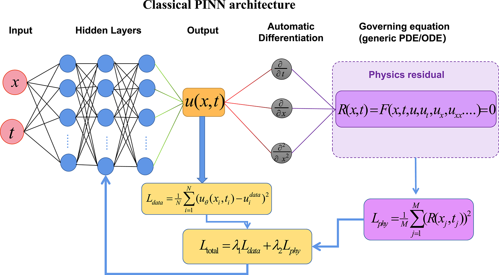
(C) Zhang, P., Zhang, H., Zhou, J. et al., Sci Rep. 16, 12760, 2026 Natural
Certain content was co-constructed with the support of a generative AI tool then reread and validated by the teacher.
from validation.libIA_GPU import Init_torchGPU

try: cuda_dev
except NameError: cuda_dev = Init_torchGPU(4, 0)
if cuda_dev is None: cuda_dev = "cpu"
print(cuda_dev)
Max threads : 4 / used threads 4
Attention: no GPU available! using CPU
cpu
/home/buffat/venvs/jupyter/lib/python3.10/site-packages/torch/cuda/__init__.py:107: UserWarning: CUDA initialization: The NVIDIA driver on your system is too old (found version 9010). Please update your GPU driver by downloading and installing a new version from the URL: http://www.nvidia.com/Download/index.aspx Alternatively, go to: https://pytorch.org to install a PyTorch version that has been compiled with your version of the CUDA driver. (Triggered internally at ../c10/cuda/CUDAFunctions.cpp:109.)
  return torch._C._cuda_getDeviceCount() > 0
Physics-Informed Neural Networks (PINN) are a method which consists of training a neural network not only on data, but also on physical laws described by differential equations. The idea was popularized by Maziar Raissi and his collaborators in 2019 Raissi, Perdikaris, and Karniadakis [2019].
references
import numpy as np
import matplotlib.pyplot as plt
import torch
import torch.nn as nn

print(torch.cuda.is_available())
device = torch.device(cuda_dev)
print("CUDA device:",cuda_dev)
print("Torch CUDA device:",device," threads:",torch.get_num_threads(),torch.get_num_interop_threads())
False
CUDA device: cpu
Torch CUDA device: cpu  threads: 4 4
10.1. Function approximation#
Function approximation is one of the fundamental applications of neural networks. With PyTorch, it’s simple to build a network that can learn a function from data.
Let’s take an example where we want to approximate the function: \(f(x)=sin(x)\)
We define the data xdata and ydata
import torch
import torch.nn as nn
import matplotlib.pyplot as plt
# Training data: attention without gradient
Nd = 100
xdata = torch.linspace(-2 * torch.pi, 2 * torch.pi, Nd,device=device).reshape(-1, 1)
ydata = torch.sin(xdata)
# neural network
class NeuralNet(nn.Module):
    def __init__(self):
        super().__init__()
        self.model = nn.Sequential(
            nn.Linear(1, 32),
            nn.Tanh(),
            nn.Linear(32, 32),
            nn.Tanh(),
            nn.Linear(32, 1)
        )
    def forward(self, x):
        return self.model(x)

model = NeuralNet().to(device)
# cost function
criterion = nn.MSELoss()
optimizer = torch.optim.Adam(model.parameters(), lr=0.01)
# network training
num_trainable = sum(p.numel() for p in model.parameters() if p.requires_grad)
print(f"Model Trainable parameters: {num_trainable}")
epochs = 3000
for epoch in range(epochs):
    optimizer.zero_grad()
    ypred = model(xdata)
    loss = torch.mean((ypred-ydata)**2)
    loss.backward()
    optimizer.step()
    if epoch % 200 == 0:
        print(f"Epoch {epoch} : Loss = {loss.item():.6f}")
print(f"Erreur finale = {loss.item():.6f}")
Model Trainable parameters: 1153
Epoch 0 : Loss = 0.571670
Epoch 200 : Loss = 0.004016
Epoch 400 : Loss = 0.000529
Epoch 600 : Loss = 0.000024
Epoch 800 : Loss = 0.000021
Epoch 1000 : Loss = 0.000008
Epoch 1200 : Loss = 0.000018
Epoch 1400 : Loss = 0.000005
Epoch 1600 : Loss = 0.000192
Epoch 1800 : Loss = 0.000003
Epoch 2000 : Loss = 0.000002
Epoch 2200 : Loss = 0.000003
Epoch 2400 : Loss = 0.000008
Epoch 2600 : Loss = 0.000002
Epoch 2800 : Loss = 0.000004
Erreur finale = 0.000213
10.1.1. Validation#
To validate, we define collocation points x (note: xdata and x are not necessarily identical).
If we want to calculate the derivatives of the function \(f(x)\), we define the collocation points x with the option x.requires_grad=True.
# collocation points where we define the function
N = 2*Nd
x = torch.linspace(-2 * torch.pi, 2 * torch.pi, N,device=device).reshape(-1, 1)
# if we want to calculate the derivatives
x.requires_grad=True
# test the model
with torch.no_grad():
    y_pred = model(x)
xn = xdata.cpu()
yn = ydata.cpu()
xp = x.detach().cpu()
yp = y_pred.cpu()
plt.figure(figsize=(8,8))
plt.subplot(2,1,1)
plt.plot(xn, yn, label="sin(x)")
plt.plot(xp, yp, '--', label="Approximation NN")
plt.legend()
plt.grid()
plt.subplot(2,1,2)
yp = model(xdata).detach().cpu()
plt.plot(xn, yn - yp)
plt.title("Erreur")
plt.show()
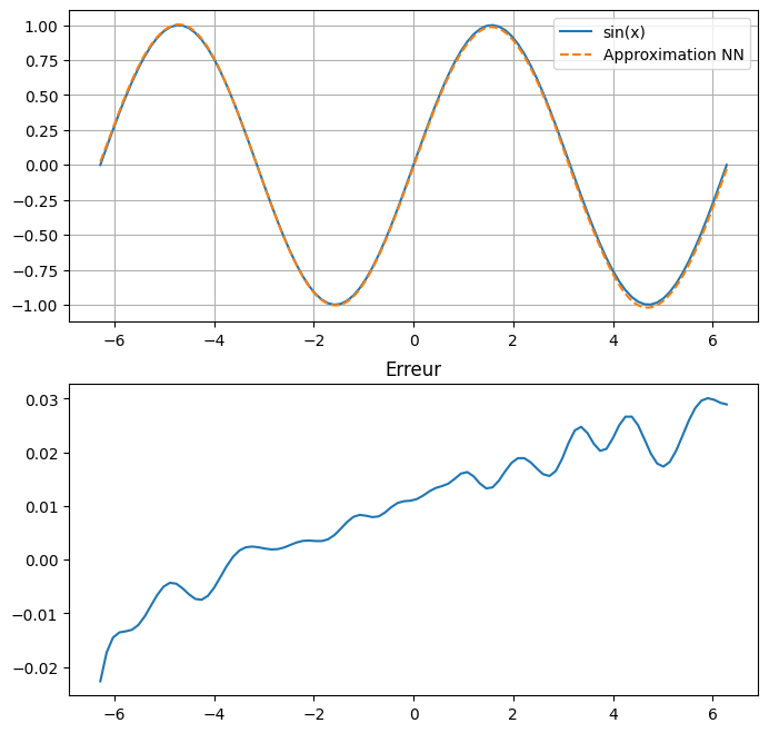
10.1.2. Calculation of the derivative#
If we calculated the approximation with x.requires_grad=True, we can calculate the derivative with the function torch.autograd.grad, which uses automatic differentiation in PyTorch.
ypred = model(x)
dypred = torch.autograd.grad(
        ypred,
        x,
        grad_outputs=torch.ones_like(ypred),
        create_graph=True
    )[0]
dyp = dypred.detach().cpu()
dye = np.cos(xp)
# trace
plt.figure(figsize=(8,8))
plt.subplot(2,1,1)
plt.title("Dérivée de la fonction $f(x)=sin(x)$")
plt.plot(xp,dyp,label='dérivée PINN')
plt.plot(xp,dye,label='exacte')
plt.legend()
plt.grid()
plt.subplot(2,1,2)
plt.plot(xp, dye - dyp)
plt.title("Erreur")
Text(0.5, 1.0, 'Erreur')
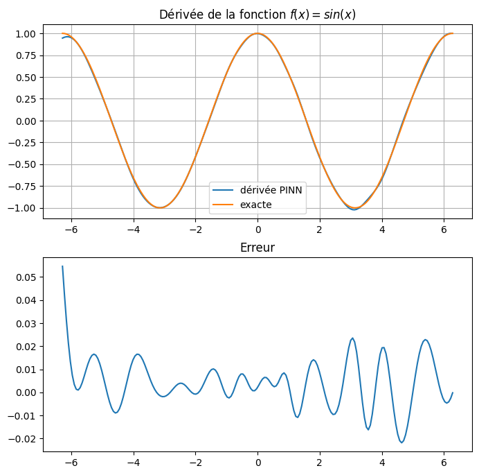
10.1.3. universal approximation theorem#
The universal approximation theorem Wikipedia states that a neural network with a sufficiently large hidden layer (with a nonlinear activation function like Tanh, ReLU or Sigmoid) can approximate any continuous function arbitrarily well on a compact domain.
Principle of nonlinear combinations
Each neuron shifts, stretches or contracts the input in a slightly different way, then passes it through a non-linear activation function to produce a partial response.
These partial responses are strongly active in some regions and almost inactive in others, like small fragments of function.
The output layer then combines these fragments by weighted sum to form the overall function.
Ultimately, the neural network does not describe a general rule in a single block: it constructs a complex function by stacking many small responses.
Meaning of approximation
The universal approximation theorem does not mean that the network always reproduces the original function exactly.
Its precise meaning is as follows: if an error tolerance is fixed in advance, it is possible to reduce the gap between functions below this tolerance.
The central idea is therefore not exactly identical, but as close as desired.
This distinction makes it possible to avoid confusing representation capacity and real precision.
with $\( \max_{x\in K} |f(x)-\hat{f}(x)| < \epsilon\)$
importance and limitation
The universal approximation theorem provides a solid mathematical basis showing that a neural network is not only a simple linear model, but can also represent extremely complex continuous functions. It is therefore often cited as a theoretical starting point to explain why Deep Learning can address a wide variety of problems.
However, this theorem only guarantees that the representation is possible: it does not mean that this representation will be effective with few neurons, nor that learning will be simple and fast. In real problems, the number of required neurons can become very large, and difficulties related to optimization, data quantity and generalization arise separately. In other words, this theorem is essential for understanding the potential of neural networks, but it does not automatically guarantee their performance in practice.
Excerpt from the ZeroMathAI program.
10.1.4. Comparison of approximation#
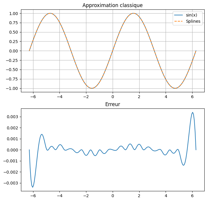
We can compare the neural network approximation with a cubic spline approximation.
In the case of the sine function, an approximation with 20 splines gives a better result than with the neural network with 1153 parameters!
It is therefore not necessary to systematically use this neural network approximation.
import numpy as np
from scipy.interpolate import CubicSpline

N = 20
x = np.linspace(-2 * np.pi, 2 * np.pi, N)
y = np.sin(x)
cs = CubicSpline(x, y)
xs = torch.linspace(-2 * np.pi, 2 * np.pi,200)
ys = np.sin(xs)
ypred = cs(xs)
plt.figure(figsize=(8,8))
plt.subplot(2,1,1)
plt.title("Approximation classique")
plt.plot(xs,ys, label="sin(x)")
plt.plot(xs,ypred, '--', label="Splines")
plt.legend()
plt.grid()
plt.subplot(2,1,2)
plt.plot(xs, ys - ypred)
plt.title("Erreur")
plt.show()
Practical advice
Normalize the data if the inputs or outputs have very different scales.
Reserve a validation set to monitor overfitting.
Choose the network capacity (number of layers and neurons) based on the complexity of the function to be approximated.
Use torch.utils.data.DataLoader for large datasets.
Monitor the loss level on the training and validation sets in order to adjust the hyper parameters (learning rate, network size, number of epochs).
This diagram forms the basis of many regression applications with PyTorch, whether to approximate an analytical function, a physical model or an empirical relationship from experimental data.
10.2. General principle of a PINN to solve an ODE#
Suppose we want to solve a differential equation
with boundary conditions or initial conditions.
Instead of discretizing the domain (as with finite difference or finite element methods), we directly approximate the solution using a neural network:
where \(\theta\) represents the network weights.
The objective is then to find the parameters \(\theta\) which make this function compatible with physical laws.
10.2.1. Using automatic differentiation#
One of the key points of PINNs is that the derivatives are calculated using the automatic differentiation of PyTorch or TensorFlow.
For example, if \(u_\theta = u_\theta(x),\) then \(\frac{\partial u_\theta}{\partial x}\) is obtained automatically by
du_dx = torch.autograd.grad(
    outputs=u,
    inputs=x,
    grad_outputs=torch.ones_like(u),
    create_graph=True
)[0]
This calculation is not based on a numerical approximation of the derivatives, but on an automatic numerical differentiation of the approximation by neural network.
10.2.2. Calculation of the physical residue#
Consider the ODE
The neural network predicts \(u_\theta(t)\). We then calculate the derivative:
then the residual of the equation
If \(u_\theta(t)\) is solution of the ODE, then \(r(t)=0 \;\forall t\)
10.2.3. Calculation Cost Function#
The training consists of minimizing several terms:
1. Physical loss
It requires the function \(u_\theta(t)\) to verify the differential equation at certain points.
The \(x_i\) are called collocation points.
2. Initial or boundary conditions
For example to impose the initial condition \(u(0)=1.\), we add
3. Experimental data (optional)
If we have some measurements \((x_i,u_i),\) we add
Thus, PINNs can work:
without data (physics alone guides learning);
with some data (hybrid case);
with a lot of data (reinforcing physical coherence).
10.2.4. Principle of the algorithm#
            Choix des points x
                  │
                  ▼
         Réseau de neurones
              uθ(x)
                  │
        ┌─────────┴──────────┐
        ▼                    ▼
 Conditions          Dérivées automatiques
initiales                 (autograd)
        │                    │
        └─────────┬──────────┘
                  ▼
          Résidu de l'équation
                  │
                  ▼
        Fonction de coût totale
                  │
                  ▼
     Descente de gradient (Adam/L-BFGS)
                  │
                  ▼
       Mise à jour des paramètres θ
10.2.5. Why does this work?#
The universal approximation theorem guarantees that a sufficiently large neural network can approximate a very large class of continuous functions. PINNs exploit this property to search for the function that best satisfies the physical equations and the imposed conditions.
10.2.6. Advantages#
No complex mesh to build.
Derivatives are obtained with high precision thanks to automatic differentiation.
Easy to extend to multidimensional problems.
Naturally integrate physical knowledge.
Can solve inverse problems, where unknown parameters are estimated along with the solution.
10.2.7. Limitations#
Training can be slow, especially for large problems. *Equations that are very steep, strongly nonlinear or with discontinuities are difficult to process.
The choice of weights between the different components of the loss function is delicate.
For many industrial PDEs, classic numerical methods (finite elements, finite volumes, finite differences) often remain faster and more precise.
In summary, a PINN replaces the traditional numerical solver with a neural network trained to directly satisfy physics equations. Solving an ODE or a PDE then becomes an optimization problem where the network parameters are adjusted to minimize the residual of the equation and respect the initial or boundary conditions.
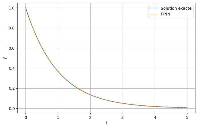
10.3. Example 1: ODE of order 1#
Here is a complete example of a Physics-Informed Neural Network (PINN) in PyTorch to solve an ordinary differential equation (ODE).
Consider the following ODE:
The analytical solution is:
The principle of a PINN is to simultaneously minimize:
the residue of the differential equation,
the initial (or boundary) conditions.
import torch
import torch.nn as nn
import matplotlib.pyplot as plt
# Device choice
print("use of",device)
#
# Neural network
#
class PINN(nn.Module):
    def __init__(self):
        super().__init__()
        self.net = nn.Sequential(
            nn.Linear(1, 32),
            nn.Tanh(),
            nn.Linear(32, 32),
            nn.Tanh(),
            nn.Linear(32, 32),
            nn.Tanh(),
            nn.Linear(32, 1)
        )

    def forward(self, x):
        return self.net(x)

model = PINN().to(device)
#
# Collocation points
#
N = 100
t = torch.linspace(0, 5, N).view(-1,1).to(device)
t.requires_grad = True
# Initial condition
t0 = torch.tensor([[0.0]], device=device)
y0 = torch.tensor([[1.0]], device=device)
optimizer = torch.optim.Adam(model.parameters(), lr=1e-3)
#
# Training
#
epochs = 5000
total_params = sum(p.numel() for p in model.parameters() if p.requires_grad)
print(f'Total number of parameters: {total_params}')

for epoch in range(epochs):
    optimizer.zero_grad()
    # Prediction
    y = model(t)
    # Derivative dy/dt
    dy_dt = torch.autograd.grad(
        outputs=y,
        inputs=t,
        grad_outputs=torch.ones_like(y),
        create_graph=True
    )[0]
    # ODE residue
    residual = dy_dt + y
    loss_ode = torch.mean(residual**2)
    # Initial condition
    pred0 = model(t0)
    loss_ic = (pred0 - y0).pow(2).mean()
    # Cost function
    loss = loss_ode + loss_ic
    # descent
    loss.backward()
    optimizer.step()
    # residue display
    if epoch % 500 == 0:
        print(f"Epoch {epoch:5d}  Loss={loss.item():.3e}")

#
# Evaluation and solution plotting
#
with torch.no_grad():
    t_test = torch.linspace(0,5,200).view(-1,1).to(device)
    y_pred = model(t_test).cpu()

t_exact = t_test.cpu()
y_exact = torch.exp(-t_exact)

plt.figure(figsize=(8,5))
plt.plot(t_exact, y_exact, label="Solution exacte")
plt.plot(t_exact, y_pred, "--", label="PINN")
plt.xlabel("t")
plt.ylabel("y")
plt.legend()
plt.grid()
plt.show()
use of cpu
Total number of parameters: 2209
Epoch     0  Loss=8.276e-01
Epoch 500 Loss=4.018e-05
Epoch 1000 Loss=1.337e-05
Epoch 1500 Loss=9.087e-06
Epoch 2000 Loss=6.050e-06
Epoch 2500 Loss=3.348e-05
Epoch 3000 Loss=6.019e-05
Epoch 3500 Loss=2.115e-06
Epoch 4000 Loss=1.509e-06
Epoch 4500 Loss=1.105e-06
10.3.1. Explanation#
The PINN learns a function \(y_\theta(t)\) parameterized by a neural network.
At each iteration:
The predicted network (y(t)).
PyTorch automatically calculates the derivative \(\frac{dy_\theta}{dt}\) thanks to
torch.autograd.grad.We construct the residue of the ODE: \(r(t)=\frac{dy_\theta}{dt}+y_\theta.\)
The loss function is $\( \mathcal{L} = \underbrace{\frac1N\sum_i r(t_i)^2}*{\text{equation}} + \underbrace{\left(y*\theta(0)-1\right)^2}_{\text{initial condition}}. \)$
The network is thus trained to simultaneously satisfy the differential equation and the initial condition.
10.3.2. Generalization#
For any ODE
just replace
residual = dy_dt + y
by
residual = dy_dt - f(t, y)
where f(t, y) is a Python function defining the right-hand side.
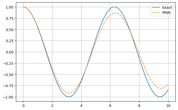
10.4. Example 2: the harmonic oscillator#
with initial conditions
The exact solution is
The idea is to have this solution learned by a PINN.
import torch
import torch.nn as nn
import matplotlib.pyplot as plt
# Device choice
print("using",device)
# =========================================================
# Neural network
# =========================================================
class PINN(nn.Module):
    def __init__(self):
        super().__init__()

        self.net = nn.Sequential(
            nn.Linear(1,64),
            nn.Tanh(),
            nn.Linear(64,64),
            nn.Tanh(),
            nn.Linear(64,64),
            nn.Tanh(),
            nn.Linear(64,1)
        )

    def forward(self,x):
        return self.net(x)

model = PINN().to(device)
# =========================================================
# Collocation points
# =========================================================
N = 200
t = torch.linspace(0,10,N).reshape(-1,1).to(device)
t.requires_grad = True

optimizer = torch.optim.Adam(model.parameters(), lr=1e-3)
# =========================================================
# Training
# =========================================================
epochs = 5000
total_params = sum(p.numel() for p in model.parameters() if p.requires_grad)
print(f'Total number of parameters: {total_params}')

for epoch in range(epochs):
    optimizer.zero_grad()
    # prediction
    y = model(t)
    # first derivative
    dy = torch.autograd.grad(
        y,
        t,
        grad_outputs=torch.ones_like(y),
        create_graph=True
    )[0]
    # second derivative
    d2y = torch.autograd.grad(
        dy,
        t,
        grad_outputs=torch.ones_like(dy),
        create_graph=True
    )[0]
    # ODE residue
    residual = d2y + y
    loss_phys = torch.mean(residual**2)
    # =========================================================
    # Initial conditions
    # =========================================================
    t0 = torch.tensor([[0.0]], requires_grad=True,device=device)
    y0 = model(t0)
    dy0 = torch.autograd.grad(
        y0,
        t0,
        grad_outputs=torch.ones_like(y0),
        create_graph=True
    )[0]
    loss_ic = (y0-1)**2 + dy0**2
    # =========================================================
    loss = loss_phys + loss_ic
    loss.backward()
    optimizer.step()
    if epoch % 500 == 0:
        print(epoch, loss.item())

# =========================================================
# verification
# =========================================================
with torch.no_grad():
    t_test = torch.linspace(0,10,300,device=device).view(-1,1)
    y_pred = model(t_test).cpu()
t_exact = t_test.cpu()
y_exact = np.cos(t_exact)

plt.figure(figsize=(8,5))
plt.plot(t_exact,y_exact,label="Exact")
plt.plot(t_exact,y_pred,"--",label="PINN")
plt.legend()
plt.grid()
plt.show()
using cpu
Total number of parameters: 8513
0 1.2456042766571045
500 0.032466258853673935
1000 0.022435003891587257
1500 0.02100544422864914
2000 0.020379532128572464
2500 0.01961708627641201
3000 0.01883835718035698
3500 0.01827062852680683
4000 0.017385432496666908
4500 0.01354198344051838
10.4.1. Explanation#
For a second order ODE, the network directly approximates the function:
The derivatives are calculated by automatic differentiation:
In PyTorch, this is done with two successive calls to torch.autograd.grad:
dy = torch.autograd.grad(
    y, t,
    grad_outputs=torch.ones_like(y),
    create_graph=True
)[0]

d2y = torch.autograd.grad(
    dy, t,
    grad_outputs=torch.ones_like(dy),
    create_graph=True
)[0]
The residue of the equation is then
and the physical loss is
The initial conditions are added in the form of penalties:
The total cost function is
10.4.2. Generalization#
For a second order ODE of the form
just replace the residue with:
residual = d2y - f(t, y, dy)
where f is a Python function. This structure is valid for most second-order ODEs, whether linear or nonlinear. It can then be extended to ODE systems by extracting several components from the network and constructing a residual for each equation.
10.5. Example 3: Reverse Problem#
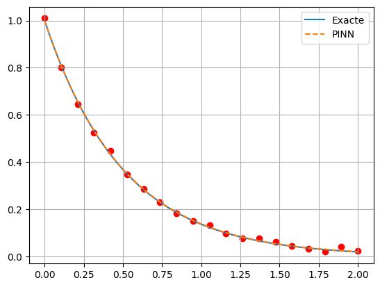
Inverse problems are one of the most interesting applications of PINNs. Unlike the direct problem (where the parameters of the equation are known), the goal here is to estimate unknown physical parameters from a few measurements.
Consider the following ODE:
with \(y(0)=1,\) where \(\lambda\) is unknown.
Suppose that we have some noisy measurements of \(y(t)\) and that we wish to find \(\lambda\).
10.5.1. Principle#
The network approximates the solution \(y_\theta(t).\)
But this time, the physical parameter is also optimized:
lambda_param = nn.Parameter(torch.tensor([0.5]))
It is added to the list of trainable parameters.
import torch
import torch.nn as nn
import matplotlib.pyplot as plt
# Device choice
print("using",device)
# =========================================================
# Data generation
# =========================================================
lambda_true = 2.0
t_data = torch.linspace(0, 2, 20,device=device).reshape(-1,1)
y_data = torch.exp(-lambda_true*t_data)
# noise
y_data += 0.01*torch.randn_like(y_data)
# =========================================================
# PINN
# =========================================================
class PINN(nn.Module):

    def __init__(self):
        super().__init__()
        self.net = nn.Sequential(
            nn.Linear(1,32),
            nn.Tanh(),
            nn.Linear(32,32),
            nn.Tanh(),
            nn.Linear(32,1)
        )

    def forward(self,x):
        return self.net(x)

model = PINN().to(device)
# =========================================================
# Unknown parameter
# =========================================================
lambda_param = nn.Parameter(torch.tensor([0.5],device=device))
# =========================================================
# Optimizer
# =========================================================
optimizer = torch.optim.Adam(
    list(model.parameters())+[lambda_param],
    lr=1e-3
)
# =========================================================
# Collocation points
# =========================================================
t_phys = torch.linspace(0,2,100,device=device).reshape(-1,1)
t_phys.requires_grad=True

# =========================================================
# Training
# =========================================================
total_params = sum(p.numel() for p in model.parameters() if p.requires_grad)
print(f'Total number of parameters: {total_params}')

for epoch in range(5000):
    optimizer.zero_grad()
    #
    # Physical
    #
    y = model(t_phys)
    dy = torch.autograd.grad(
        y,
        t_phys,
        grad_outputs=torch.ones_like(y),
        create_graph=True
    )[0]
    residual = dy + lambda_param*y
    loss_phys = torch.mean(residual**2)
    #
    # Data
    #
    y_pred = model(t_data)
    loss_data = torch.mean((y_pred-y_data)**2)
    #
    # Initial condition
    #
    t0 = torch.tensor([[0.0]],device=device)
    loss_ic = (model(t0)-1.)**2
    #
    loss = loss_phys + loss_data + loss_ic
    loss.backward()
    optimizer.step()
    if epoch%500==0:
        print(epoch,
              loss.item(),
              lambda_param.item())

print("\nEstimated value:", lambda_param.item(), "exacte:",lambda_true)

# =========================================================
# Comparison
# =========================================================
with torch.no_grad():
    t_test = torch.linspace(0,2,200,device=device).reshape(-1,1)
    y_pred = model(t_test).cpu()

t = t_test.cpu()
plt.plot(t,np.exp(-lambda_true*t),label="Exacte")
plt.plot(t,y_pred,'--',label="PINN")
plt.scatter(t_data.cpu(),y_data.cpu(),color='red')
plt.legend()
plt.grid()
plt.show()
using cpu
Total number of parameters: 1153
0 1.2559903860092163 0.49900001287460327
500 0.029163891449570656 0.9227480888366699
1000 0.01147594302892685 1.2425323724746704
1500 0.004831275437027216 1.4698596000671387
2000 0.002023914596065879 1.6394798755645752
2500 0.0008158246637322009 1.7665849924087524
3000 0.0003198199556209147 1.859109878540039
3500 0.00013796999701298773 1.9225051403045654
4000 8.311892452184111e-05 1.961584210395813
4500 7.035602902760729e-05 1.9823417663574219
Estimated value: 1.9915227890014648 exacte: 2.0
10.5.2. Explanation#
The network simultaneously learns:
the function \(y(t)\),
the \(\lambda\) parameter.
The loss function is written
with
Physical Loss
Loss of Data
Loss on the Initial Condition
10.5.3. Why does this work?#
The loss gradient depends on two types of parameters:
the weights of the neural network \(\theta\);
the physical parameter \(\lambda\).
As \(\lambda\) is declared as a nn.Parameter, PyTorch automatically calculates
and the optimizer updates \(\lambda\) exactly like the network weights.
10.6. Real-world applications of PINNs#
This approach is used to identify physical parameters from limited data, for example:
diffusion coefficient in a heat equation;
viscosity of a fluid in the Navier–Stokes equations;
Young’s modulus or thermal conductivity of a material;
reaction constants in chemical kinetics;
parameters of an epidemiological model (for example the transmission rate in an SIR model);
damping and stiffness parameters in mechanical systems.
It is precisely in this context where there are few measurements but a reliable physical model that PINNs often offer their greatest value.
10.6.1. Possible extensions#
This structure easily extends to more complex problems:
ODE systems (Lotka-Volterra, pendulum, Lorenz, etc.) by bringing several components out of the network.
Higher order differential equations, calculating successive derivatives with
torch.autograd.grad.Partial differential equations (PDE) such as the heat, Burgers or Navier-Stokes equation, using multiple input variables (
x,t, etc.) and corresponding partial derivatives.Inverse PINNs, where some physical parameters of the ODE are also learned by the network by declaring them as optimizable parameters (
torch.nn.Parameter).