Théorie de l’aile

Marc BUFFAT département mécanique, Lyon 1

%matplotlib inline
import numpy as np
import sympy as sp
import matplotlib.pyplot as plt

from metakernel import register_ipython_magics
register_ipython_magics()

Théorie de la portance¶

les différentes théories de la portance (sur internet):

Appuie de l’aile sur l’air (principe de réaction de Newton)
Bernoulli + égalité des temps de parcours
Analyse globale: bilan de quantité de mouvement, déviation de l’écoulement
Théorie de la Circulation de vitesse

lien vers le sondage sur https://l3-nbgrader/Survey/MGC3062L

#%activity /usr/local/commun/ACTIVITY/MGC3062L/portance

UsageError: Line magic function `%activity` not found.

Caractéristique aérodynamique d’un profil¶

Analyse dimensionnelle:

Etude d’un profil 2D

étude en fonction de l’angle $\alpha$
fonction du nombre de Reynolds
$C_L$ coefficiant de portance: projection suivant $\vec{N}=[-\sin\alpha, \cos\alpha]$ $\perp$ à $\vec{U}_0$

C_L = \int_{C} Pr\, \vec{n}.\vec{N}\,ds

(1)

C_L = \int_{C} Pr\, ds \mbox{ avec } ds = dx \cos{\alpha} + dy \sin{\alpha}

(2)

$C_m$ coefficient de moment (moment pression) par rapport à un point de référence $P=[x_{ref}=0.25, y_{ref}=0]$ , qui n’est donc pas nécessairement sur la ligne moyenne à 1/4 de corde

C_m = \int_{C} Pr\, \vec{n} \land \vec{PM} \,ds

(3)

C_m = \int_{C} -Pr \left((x-x_{ref}) dx + (y-y_{ref}) dy \right)

(4)

on calcule alors le moment en un point Q quelconque par la relation de transport

\mathcal{M}_Q = \mathcal{M}_P + \vec{QP} \land \vec{F}_p \mbox{ avec } \vec{F}_p = C_L [-\sin\alpha, \cos\alpha]

(5)

d’où la position du centre de poussée exacte / à $P$ $x,y$ (erreur)

\frac{C_m}{C_L} = (x- x_{ref})\cos\alpha + (y- y_{ref})\sin\alpha

(6)

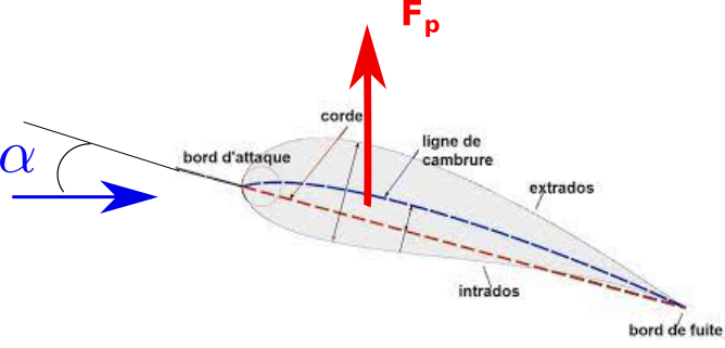
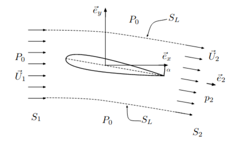
Analyse par bilan de quantité de mouvement¶

Modèle simplifié des efforts exercés par un profil d’aile de longueur (de corde) $L_c$ en incidence d’angle $\alpha$ sur un écoulement stationnaire d’un fluide parfait incompressible de masse volumique $\rho$ et de vitesse $U_1$ (schéma ci-dessous)

On constate expérimentalement que l’effet de l’aile sur l’écoulement, aux faibles incidences, est de dévier les lignes de courant d’un angle $\alpha$ correspondant à l’angle d’incidence du profil, c.a.d l’angle d’inclinaison du bord de fuite.

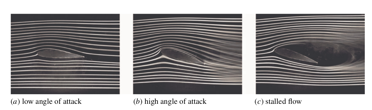
d’après “How do wings work?” H. Babinsky, Physics Education 38(6) 2003

A 1-minute video released by the University of Cambridge sets the record straight on a much misunderstood concept - how wings lift. I start by giving the wrong explanation and asking who has heard it and every time 95% of the audience puts their hand up. Only a handful will know that it is wrong.Professor Holger BabinskyIt’s one of the most tenacious myths in physics and it frustrates aerodynamicists the world over. Now, …

from IPython.display import YouTubeVideo

YouTubeVideo('e0l31p6RIaY', width=600, height=400)

Loading...

bilan de masse et de quantité de mouvement¶

$U_1 S_1 = U_2 S_2$
(7)
$p_1 = p_2 = p_0$
(8)
$S_2 = L_c W$
(9)

on en déduit par bilan de quantité de mouvement la force de portance et le coefficient de portance $C_p$

Fp = \rho U_1^2 \sin\alpha W L_c

(10)

soit à faible incidence une proportionnalité du coefficient de portance $C_p$ avec l’angle d’incidence $\alpha$

C_p = \frac{F_p}{\rho U_1^2 W L_c} \approx \alpha

(11)

Potentiel complexe¶

Pour un écoulement incompressible 2D de fluide parfait irrotationnel le potentiel $\phi(x,y)$ et la fonction de courant $\psi(x,y)$ vérifie l’éuqtaion de Laplace:

\Delta \psi = \Delta \phi = 0

(12)

dont le champ de vitesse $\vec{U} = [U_x,U_y]$ en cartésien est donné par

U_x = \frac{\partial \phi}{\partial x} = \frac{\partial \psi}{\partial y}

(13)

U_y = \frac{\partial \phi}{\partial y} = -\frac{\partial \psi}{\partial x}

(14)

On définit alors un potentiel complexe $\Phi(z)$ :

\Psi(z) = \phi(x,y) + i \psi(x,y)

(15)

qui est une fonction analytique en z, dont la dérivée est indépendante de dz.

Dans ce cas $\Phi(z)$ est différentiable en z et vérifie:

\begin{align*} \frac{d \Phi}{d z} &= \frac{\partial \phi}{\partial x} + i \frac{\partial \psi}{\partial x}\\ &= -i \frac{\partial \phi}{\partial y} + \frac{\partial \psi}{\partial y}\\ &= U_x - i U_y \\ \end{align*}

(16)

On le vérifie en prenant respectivement $\delta z = \delta x$ et $\delta z = i\delta y$ et en utilisant les relations de Cauchy-Riemann entre $\phi$ et $\psi$

On en déduit le module de la vitesse:

\| U \| = \sqrt{U_x^2+U_y^2} = \left|\frac{d \Psi}{d z}\right|

(17)

et son angle $\theta$

\theta = -arg\left(\frac{d \Psi}{d z} \right)

(18)

Coordonnées polaires¶

En coordonnées polaires, l’équation de Laplace s’écrit:

\frac{1}{r}\frac{\partial }{\partial r} \left(r \frac{\partial \Psi}{\partial r} \right) + \frac{1}{r^2}\frac{\partial^2 \Psi}{\partial r^2} = 0

(19)

et le champ de vitesse en polaire

U_r = \frac{\partial \Phi}{\partial r} \mbox{ et } U_\theta = \frac{1}{r} \frac{\partial \Phi}{\partial \theta}

(20)

U_r = \frac{1}{r} \frac{\partial \Psi}{\partial \theta} \mbox{ et } U_\theta = -\frac{\partial \Psi}{\partial r}

(21)

soit en coordonnées cartésiennes

U_x = U_r \cos\theta - U_\theta \sin \theta \mbox{ et } U_y = U_r \sin\theta + U_\theta \cos \theta

(22)

Potentiel complexe en polaire¶

puisque $z = r e^{i\theta}$ on a donc :

\begin{align*} \frac{d \Phi}{d z} &= \frac{\partial \phi}{\partial r} e^{-i\theta} + i \frac{\partial \psi}{\partial r} e^{-i\theta}\\ &= -\frac{i}{r}\frac{\partial \phi}{\partial \theta}e^{-i\theta} + \frac{1}{r}\frac{\partial \psi}{\partial \theta}e^{-i\theta}\\ &= U_x -i U_y = (U_r - i U_\theta) e^{-i\theta} \\ \end{align*}

(23)

avec

U_r = U_x \cos \theta + U_y \sin \theta \mbox{ et } U_\theta = -U_x \sin \theta + U_y \cos \theta

(24)

On en déduit aussi

\begin{align*} \frac{\partial \Phi}{\partial r} &= \frac{\partial \phi}{\partial r} + i \frac{\partial \psi}{\partial r}\\ &= U_r - i U_\theta \end{align*}

(25)

Potentiel complexe de l’écoulement autour d’un cylindre¶

On a vu que l’écoulement potentiel autour d’un cylindre de rayon $R$ en rotation est la somme d’un écoulement uniforme, d’un doublet et d’un vortex de circulation $\Gamma$

Pour une vitesse $U_0$ d’incidence $\alpha$ , le potentiel complexe s’écrit

\Psi(z) = U_0 z e^{-i\alpha} + U_0 e^{i\alpha} \frac{R^2}{z} - i \frac{\Gamma}{2\pi}\log(\frac{z e^{-i\alpha}}{R})

(26)

et la vitesse complexe $W = U- i V$

W = U_0 e^{-i\alpha} - U_0 e^{i\alpha} \frac{R^2}{z^2} - i \frac{\Gamma}{2\pi z}

(27)

# parametres
R, U0 = sp.symbols('R U_0',real=True, positive=True)
Gamma,alpha = sp.symbols('Gamma alpha',real=True)
# variables
theta,x,y = sp.symbols('theta x y',real=True)
r         = sp.symbols('r',real=True,Positive=True)
# fonctions pour manipuler les complexes
from sympy import re,im,I

Pour une vitesse $U_0$ d’incidence $\alpha$ , le potentiel complexe s’écrit

\Psi(z) = U_0 z e^{-i\alpha} + U_0 e^{i\alpha} \frac{R^2}{z} - i \frac{\Gamma}{2\pi}\log(\frac{z e^{-i\alpha}}{R})

(28)

# potentiel complexe Phi
z = sp.symbols('z')
Phi = U0*z*sp.exp(-I*alpha) + U0*sp.exp(I*alpha)*R**2/z \
    - (I*Gamma/(2*sp.pi))*sp.log(z*sp.exp(-I*alpha)/R)
display("Phi(z)=",Phi)

'Phi(z)='

Loading...

la vitesse complexe $W = U- i V$ est alors donnée par

W = \frac{d \Phi}{d z}

(29)

# calcul de la vitesse complexe W
W = 0
### BEGIN SOLUTION
W = sp.diff(Phi,z)
### END SOLUTION
display("W(z)=",W)

'W(z)='

Loading...

# calcul fonction de courant psi (en fonction de (x,y)
psi = 0
### BEGIN SOLUTION
psi = im(Phi.subs(z,x+sp.I*y))
### END SOLUTION
display('psi(x,y)=',psi)

'psi(x,y)='

Loading...

# en déduire les composantes de vitesse dans Ux et Uy
Ux = 0
Uy = 0
### BEGIN SOLUTION
Ux =  re(W.subs(z,x+sp.I*y))
Uy = -im(W.subs(z,x+sp.I*y))
### END SOLUTION
display("Ux=",Ux)
display("Uy=",Uy)

'Ux='

Loading...

'Uy='

Loading...

Visualisation des champs¶

utilisation d’une technique de masque pour éliminer l’écoulement à l’intérieur du cercle

# parametres numeriques: choix arbitraire de Gamma et alpha ! 
R0   = 0.5
Uinf = 1.0
vals = [(Gamma,-2*np.pi*R*U0),(alpha,np.deg2rad(10)),(R,R0),(U0,Uinf)]
display("parametres:",vals)

'parametres:'

[(Gamma, -6.28318530717959*R*U_0),
 (alpha, 0.17453292519943295),
 (R, 0.5),
 (U_0, 1.0)]

# domaine de calcul et maillage (grille) pour le calcul de psi et de la vitesse
L = 3
N = 201
pas = 8 # pas pour les vitesses
# points de calcul
xg = np.linspace(-L,L,N)
yg = np.linspace(-L/2,L/2,N)
# pour les lignes de courant psi
X, Y = np.meshgrid(xg, yg)
# utilisation d'un masque
Z = X + 1j*Y
Z = np.ma.masked_where(np.absolute(Z)<0.95*R0,Z)
X = Z.real
Y = Z.imag
# et le champ de vitesse U
XX = X[::pas,::pas]
YY = Y[::pas,::pas]

# calcul des valeurs numeriques
psi1 = sp.lambdify([x,y],psi.subs(vals),'numpy')
u1   = sp.lambdify([x,y],Ux.subs(vals),'numpy')
v1   = sp.lambdify([x,y],Uy.subs(vals),'numpy')
with np.errstate(divide='ignore'):
    Psi1 = psi1(X,Y)
    Psi0 = psi1(0.5,0)
    Levs = np.linspace(Psi0-L/5,Psi0+L/5,21)
    U1   = u1(XX,YY)
    V1   = v1(XX,YY)

<lambdifygenerated-1>:2: RuntimeWarning: invalid value encountered in sqrt
  return -0.17364817766693*x + 0.984807753012208*y + 1.5707963267949*log(2.0*sqrt(x**2 + y**2))/pi + 0.25*imag(exp(0.174532925199433*1j)/(x + 1j*y))

# tracer
fig, ax = plt.subplots(figsize=(12,6))
#ax.contourf(X,Y,Psi1,levels=21)
ax.contour(X,Y, Psi1,levels=Levs,colors='r')
ax.quiver(XX,YY,U1,V1)
cercle = plt.Circle((0.,0.),R0,color='yellow')
ax.add_artist(cercle)
plt.axis('equal')
plt.axis('off')
plt.title("Ecoulement autour du cylindre");

Transformation conforme¶

On définit une transformation conforme $Z=F(z)$ qui préserve les angles dans le plan complexe.

Transformation de Joukovski¶

Z = z + \frac{C^2}{z}

(30)

avec $z = x + i y$ (plan d’origine) et $Z = X + i Y$ (plan transformé)

C = sp.symbols('C',real=True,positive=True)
F = lambda z: z + C**2/z
display("Z=F(z)",F(z))

'Z=F(z)'

Loading...

transformation conforme¶

transformation de l’écoulement autour d’un cercle de centre $x0,y0$ de rayon $R=R_0$

$c$ paramétre de la transformation $0\le c\le 1$
$\beta$ angle du point centre / horizontal

# selection cas 1,2,3,4 (choix 4 par defaut)
cas  = 4
beta = 0
if cas==0:
    # cercle
    x0 = 0
    y0 = 0
    R0 = float(R.subs(vals))
    c  = float(R.subs(vals)*0.0)
elif cas==1:
    # parametres pour une ellipse
    x0 = 0
    y0 = 0
    R0 = float(R.subs(vals))
    c  = float(R.subs(vals)*0.9)
elif cas==2:
    # parametre pour une plaque
    x0 = 0
    y0 = 0
    R0 = float(R.subs(vals))
    c  = float(R.subs(vals)*1.0)
elif cas==3:
    # parametres pour un profil symetrique
    R0 = float(R.subs(vals))
    c  = float(R.subs(vals)/1.2) 
    x0 = c - R0
    y0 = 0
else:
    # parametres pour un profil cambre
    beta = np.deg2rad(8)
    R0 = float(R.subs(vals))
    c  = float(R.subs(vals)/1.2)
    x0 = c - R0*np.cos(beta)
    y0 = R0*np.sin(beta)

# calcul de la transformation en coordonnées cartésienne
xc = re(F(x+sp.I*y))
yc = im(F(x+sp.I*y))
display("xc,yc=",xc,yc)

'xc,yc='

Loading...

# transformation du cercle
Xc = sp.lambdify([x,y],xc.subs(C,c),'numpy')
Yc = sp.lambdify([x,y],yc.subs(C,c),'numpy')
Theta = np.linspace(0,2*np.pi,410)
XC = Xc(x0+R0*np.cos(Theta),y0+R0*np.sin(Theta))
YC = Yc(x0+R0*np.cos(Theta),y0+R0*np.sin(Theta))

plt.figure(figsize=(8,6))
plt.plot(XC,YC)
plt.title("Transformation de Joukovski")
plt.axis('equal');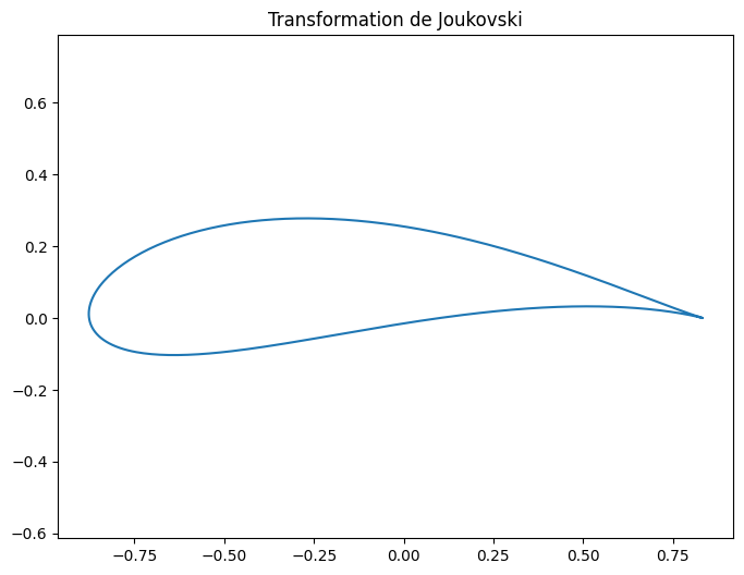

calcul de l’écoulement par transformation de Joukovski¶

calcul pour un profil
transformation numérique

def TransJ(Z,lam):
    '''transformation Joukovski (complexe)'''
    return Z + lam**2/Z
def Cercle(C0,R):
    '''pts du cercle de centre C0 (complexe) et de rayon R'''
    Theta = np.linspace(0,2*np.pi,200)
    return C0 + R*np.exp(1j*Theta)

def solutionJ(PHI,lam,C0,R,xg,yg):
    '''calcul de la solution par transformation de Joukovski PHI'''
    X,Y  = np.meshgrid(xg,yg)
    Z    = X+1j*Y
    Z    = np.ma.masked_where(np.absolute(Z-C0)<=R,Z)
    Zc   = Z - C0
    #Phiz = PHI(Z)
    # BUG numpy: calcul 
    # np.log(Z) cannot be calculated correctly due to a numpy bug np.log(MaskedArray);
    Phiz = Zc.copy()
    with np.errstate(divide='ignore'):        
        for m in range(Zc.shape[0]):
            for n in range(Zc.shape[1]):
                Phiz[m,n] = PHI(Zc[m,n])
    # Joukovski transformation 
    J  = TransJ(Z, lam)  
    cercle = Cercle(C0, R)
    airfoil= TransJ(cercle, lam) 
    return J, Phiz.imag, airfoil

#valeur des  parametres
display("parametres ",vals)
alpha0 = np.rad2deg(float(alpha.subs(vals)))
print("alpha={} deg. beta={} deg. c={} C0={}".format(alpha0,np.rad2deg(beta),c,x0+1j*y0))

'parametres '

[(Gamma, -6.28318530717959*R*U_0),
 (alpha, 0.17453292519943295),
 (R, 0.5),
 (U_0, 1.0)]

alpha=10.0 deg. beta=8.0 deg. c=0.4166666666666667 C0=(-0.0784673677041185+0.06958655048003272j)

display(Phi)
# calcul du potentiel complexe 
PhiJ = Phi.subs(vals)
display("Phi(z)=",PhiJ)
# conversion fonction python
PHI  = sp.lambdify(z,PhiJ)

Loading...

'Phi(z)='

Loading...

# calcul solution ! pble mauvaise valeur de la circulation 
J, Psi, airfoil = solutionJ(PHI,c,x0+1j*y0,R0,xg,yg)
# tracer
fig=plt.figure(figsize=(12,8))
ax=fig.add_subplot(111)
# this means that the flow is evaluated at Juc(z) since c_flow(Z)=C_flow(csi(Z))
cp=ax.contour(J.real, J.imag, Psi,levels=Levs, colors='blue', linewidths=1,
                linestyles='solid')
ax.plot(airfoil.real, airfoil.imag)
ax.fill(airfoil.real, airfoil.imag,color='yellow')
plt.axis('off')
plt.title("Problème: eclt au bord de fuite car circulation non correcte")
ax.set_aspect('equal');
#plt.savefig('eclt_cylindre.png')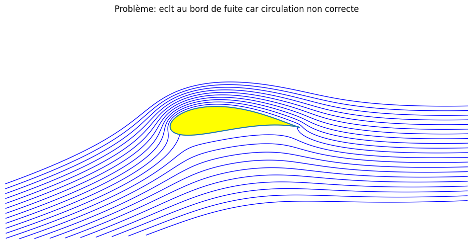

circulation de Kutta-Joukovsky¶

condition de Kutta au bord de fuite !

\Gamma = -4 \pi U_0 R \sin{(\alpha + \beta)}

(31)

# valeur de Joukovski
GammaJ = -4*sp.pi*U0*R*sp.sin(alpha+beta)
display("GammaJ=",GammaJ)
# potentiel Joukovsky
PhiJ = Phi.subs(Gamma,GammaJ).subs(vals)
display("PhiJ=",PhiJ)
# conversion fonction python
PHI  = sp.lambdify(z,PhiJ)

'GammaJ='

Loading...

'PhiJ='

Loading...

# calcul solution
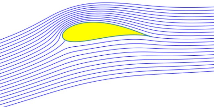
J, Psi, airfoil = solutionJ(PHI,c,x0+1j*y0,R0,xg,yg)
# tracer
fig=plt.figure(figsize=(12,8))
ax=fig.add_subplot(111)
# this means that the flow is evaluated at Juc(z) since c_flow(Z)=C_flow(csi(Z))
cp=ax.contour(J.real, J.imag, Psi,levels=Levs, colors='blue', linewidths=1,
                linestyles='solid')
ax.plot(airfoil.real, airfoil.imag)
ax.fill(airfoil.real, airfoil.imag,color='yellow')
plt.axis('off')
ax.set_aspect('equal');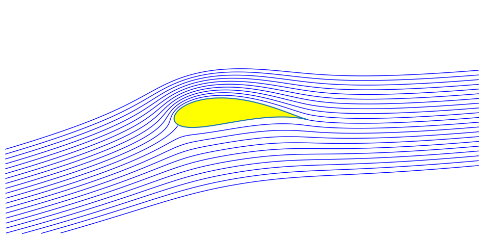

Calcul de la Portance¶

Condition de Kutta - Joukovsky¶

création circulation vitesse $\Gamma$ telle que la vitesse reste parallèle au bord de fuite (pas de contournement)

condition de kutta-joukovski

circulation

\Gamma = 4 \pi U_0 R_0 \sin(\alpha + \beta)

(32)

portance

F_p = \rho \Gamma U_0

(33)

en faible incidence

F_p \propto (\alpha + \beta)

(34)

Expérience de Prandtl (~1918)¶

création de la circulation

from IPython.display import YouTubeVideo

YouTubeVideo('VcggiVSf5F8', width=600, height=400)

Loading...

Annexe: Joukovski-airfoil¶

Ce notebook est inspiré d’un notebook de calcul de l’écoulement autour d’un profil de Joukovski

Théorie de la portance¶

Caractéristique aérodynamique d’un profil¶

Analyse par bilan de quantité de mouvement¶

bilan de masse et de quantité de mouvement¶

Potentiel complexe¶

Coordonnées polaires¶

Potentiel complexe en polaire¶

Potentiel complexe de l’écoulement autour d’un cylindre¶

Visualisation des champs¶

Transformation conforme¶

Transformation de Joukovski¶

transformation conforme¶

calcul de l’écoulement par transformation de Joukovski¶

circulation de Kutta-Joukovsky¶

Calcul de la Portance¶

Condition de Kutta - Joukovsky¶

Expérience de Prandtl (~1918)¶

Annexe: Joukovski-airfoil¶

FIN¶