Écoulement à surface libre January 1, 2012
objectifs : appréhender les domaines de l’hydraulique, hydrodynamique maritime et la notion d’ondes de surface
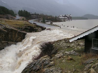
Figure 1: crue de rivière
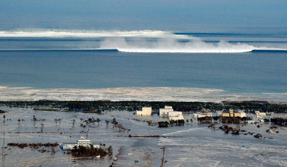
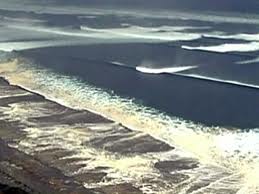
Figure 2: tsunami au japon
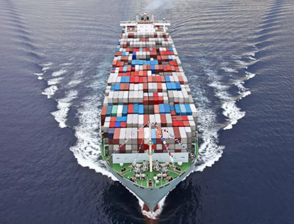
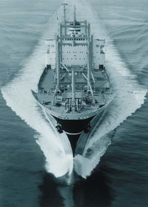
Figure 3: sillage à l’arrière d’un bateau
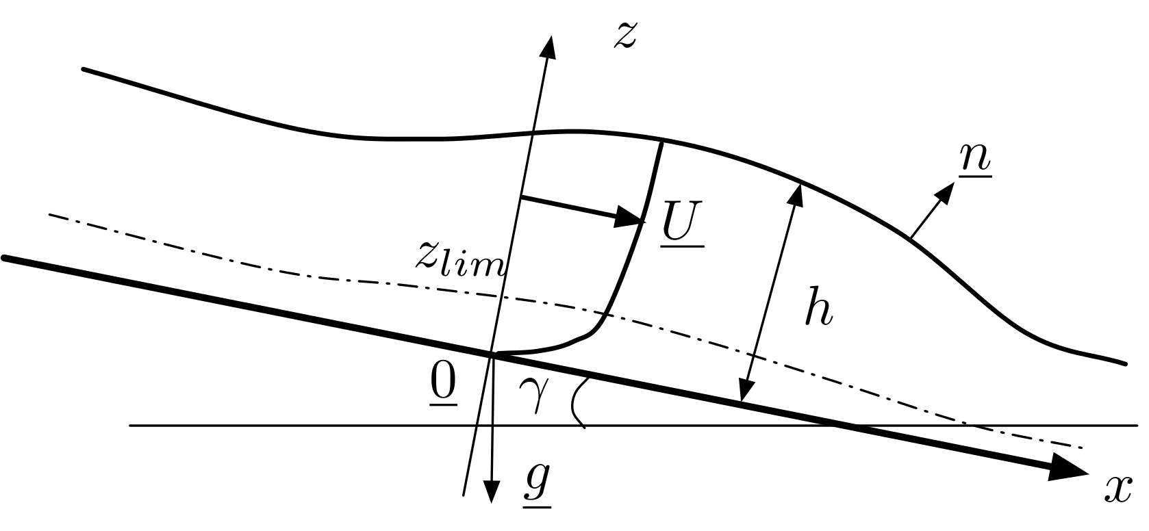
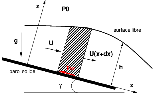
Modèle en eau peu profonde (rivière) ¶ fluide incompressible (eau), effet de gravité, surface libre, faible
profondeur
Figure 4: modèle en eau peu profonde
Équations de Navier-Stokes en 2D U → = ( u , v ) \overrightarrow{U}=(u,v) U = ( u , v )
d i v ( U → ) = 0 ∂ ρ U → ∂ t + d i v ( ρ U → ⊗ U → ) = − ∇ → p + ρ g → + μ Δ U → \begin{aligned}
div(\overrightarrow{U}) & =0\\
\frac{\partial\rho\overrightarrow{U}}{\partial t}+div\left(\rho\overrightarrow{U}\otimes\overrightarrow{U}\right) & =-\overrightarrow{\nabla}p+\rho\overrightarrow{g}+\mu\Delta\overrightarrow{U}\end{aligned} d i v ( U ) ∂ t ∂ ρ U + d i v ( ρ U ⊗ U ) = 0 = − ∇ p + ρ g + μ Δ U paramétres: U 0 U_{0} U 0 L L L τ 0 \tau_{0} τ 0 h h h g g g γ \gamma γ μ \mu μ ρ \rho ρ
5 nombres sans dimension
R e = ρ U 0 h μ , F r = U 0 g h , γ , ϵ = h L , S t = U 0 τ 0 L Re=\frac{\rho U_{0}h}{\mu},\,\,Fr=\frac{U_{0}}{\sqrt{gh}},\,\,\gamma,\,\,\epsilon=\frac{h}{L},\,St=\frac{U_{0}\tau_{0}}{L} R e = μ ρ U 0 h , F r = g h U 0 , γ , ϵ = L h , St = L U 0 τ 0 l’échelle de vitesse suivant z z z W 0 ≈ ϵ U 0 W_{0}\approx\epsilon U_{0} W 0 ≈ ϵ U 0
exemple:
μ = 1 0 − 3 P a s \mu=10^{-3}\,Pa\,s μ = 1 0 − 3 P a s ρ = 1 0 3 k g / m 3 \rho=10^{3}\,kg/m^{3} ρ = 1 0 3 k g / m 3 U 0 = 1 − 10 m / s U_{0}=1-10m/s U 0 = 1 − 10 m / s h ∼ 1 m h\sim1\,m h ∼ 1 m L ≈ k m L\approx km L ≈ km
R e ∼ 1 0 6 − 1 0 7 , F r ∼ 0.3 − 3 Re\sim10^{6}-10^{7},\,\,Fr\sim0.3-3 R e ∼ 1 0 6 − 1 0 7 , F r ∼ 0.3 − 3 hypothèses :
p = P 0 + ρ g cos ( γ ) ( h − z ) p=P_{0}+\rho g\cos(\gamma)(h-z) p = P 0 + ρ g cos ( γ ) ( h − z ) Figure 5: modèle de Saint Venant
Bilan de masse sur une tranche de fluide h d x d y hdxdy h d x d y
Δ ρ h d x d y Δ t − ρ U x h x d y + ρ U x + d x h x + d x d y = 0 \frac{\Delta\rho hdxdy}{\Delta t}-\rho U_{x}h_{x}dy+\rho U_{x+dx}h_{x+dx}dy=0 Δ t Δ ρ h d x d y − ρ U x h x d y + ρ U x + d x h x + d x d y = 0 DL à l’ordre 1:
∂ h ∂ t + ∂ h U ∂ x = 0 \frac{\partial h}{\partial t}+\frac{\partial hU}{\partial x}=0 ∂ t ∂ h + ∂ x ∂ h U = 0 bilan de quantité de mouvement sur une tranche de fluide h d x d y hdxdy h d x d y
Δ ρ U h d x d y Δ t + ρ ( U 2 h x + d x − U 2 h x ) d x d y = ( − Δ ( p ‾ h ) + P 0 Δ h ) d y + ( ρ g h sin γ − τ w ) d x d y \frac{\Delta\rho Uhdxdy}{\Delta t}+\rho\left(U^{2}h_{x+dx}-U^{2}h_{x}\right)dxdy=\left(-\Delta(\overline{p}h)+P_{0}\Delta h\right)dy+\left(\rho gh\sin\gamma-\tau_{w}\right)dxdy Δ t Δ ρ U h d x d y + ρ ( U 2 h x + d x − U 2 h x ) d x d y = ( − Δ ( p h ) + P 0 Δ h ) d y + ( ρ g h sin γ − τ w ) d x d y répartition de pression hydrostatique suivant z z z
p = P 0 + ρ g cos ( γ ) ( h − z ) ⟹ p ‾ = P 0 + ρ g cos ( γ ) h 2 p=P_{0}+\rho g\cos(\gamma)(h-z)\Longrightarrow\overline{p}=P_{0}+\rho g\cos(\gamma)\frac{h}{2} p = P 0 + ρ g cos ( γ ) ( h − z ) ⟹ p = P 0 + ρ g cos ( γ ) 2 h DL à l’ordre 1 avec τ w = C f ρ U 2 \tau_{w}=C_{f}\rho U^{2} τ w = C f ρ U 2
∂ U h ∂ t + ∂ U 2 h ∂ x = − g cos ( γ ) h ∂ h ∂ x + g h sin ( γ ) − C f U 2 \frac{\partial Uh}{\partial t}+\frac{\partial U^{2}h}{\partial x}=-g\cos(\gamma)h\frac{\partial h}{\partial x}+gh\sin(\gamma)-C_{f}U^{2} ∂ t ∂ U h + ∂ x ∂ U 2 h = − g cos ( γ ) h ∂ x ∂ h + g h sin ( γ ) − C f U 2 si l’angle est petit: γ ≪ 1 \gamma\ll 1 γ ≪ 1
∂ U h ∂ t + ∂ U 2 h ∂ x = γ g h − g h ∂ h ∂ x − C f U 2 \frac{\partial Uh}{\partial t}+\frac{\partial U^{2}h}{\partial x}=\gamma gh-gh\frac{\partial h}{\partial x}-C_{f}U^{2} ∂ t ∂ U h + ∂ x ∂ U 2 h = γ g h − g h ∂ x ∂ h − C f U 2 On obtiens aisni les équation de St Venant, du nom de Adhémar-Jean-Claude Barré de Saint-Venant (ingénieur mathématicien français 1797-1886)
écoulement de vitesse moyenne
U → ( x , t ) = U e x → \overrightarrow{U}(x,t)=U\overrightarrow{e_{x}} U ( x , t ) = U e x h ( x ) h(x) h ( x )
∂ h ∂ t + ∂ h U ∂ x = 0 ∂ h U ∂ t + ∂ U 2 h ∂ x = γ g h − g h ∂ h ∂ x − C f U 2 \begin{aligned}
\frac{\partial h}{\partial t}+\frac{\partial hU}{\partial x} & =0\\
\frac{\partial hU}{\partial t}+\frac{\partial U^{2}h}{\partial x} & =\gamma gh-gh\frac{\partial h}{\partial x}-C_{f}U^{2}\end{aligned} ∂ t ∂ h + ∂ x ∂ h U ∂ t ∂ h U + ∂ x ∂ U 2 h = 0 = γ g h − g h ∂ x ∂ h − C f U 2 remarque: on peut les obtenir par dérivation à partir de Navier-Stokes en considérant les moyennes
U ( x , t ) = 1 h ∫ 0 h u ( x , z , t ) d z U(x,t)=\frac{1}{h}\int_{_{0}}^{h}u(x,z,t)dz U ( x , t ) = h 1 ∫ 0 h u ( x , z , t ) d z écoulement de vitesse moyenne
U → ( x , y ) = U e x → + V e y → \overrightarrow{U}(x,y)=U\overrightarrow{e_{x}}+V\overrightarrow{e_{y}} U ( x , y ) = U e x + V e y h ( x , y ) h(x,y) h ( x , y )
∂ h ∂ t + d i v ( h U → ) = 0 ∂ h U → ∂ t + d i v ( h U → ⊗ U → ) = γ g h − g h g r a d → h − C f ∣ U ∣ U → \begin{aligned}
\frac{\partial h}{\partial t}+div(h\overrightarrow{U}) & =0\\
\frac{\partial h\overrightarrow{U}}{\partial t}+div(h\overrightarrow{U}\otimes\overrightarrow{U}) & =\gamma gh-gh\,\overrightarrow{grad}h-C_{f}\left|U\right|\,\overrightarrow{U}\end{aligned} ∂ t ∂ h + d i v ( h U ) ∂ t ∂ h U + d i v ( h U ⊗ U ) = 0 = γ g h − g h g r a d h − C f ∣ U ∣ U le moteur de l’écoulement est la gravité qui compense le frottement au
fond:
γ g h 0 ∼ C f U 0 2 \gamma gh_{0}\sim C_{f}U_{0}^{2} γ g h 0 ∼ C f U 0 2 Les nombres sans dimension importants sont:
F r = U 0 g h 0 Fr=\frac{U_{0}}{\sqrt{gh_{0}}} F r = g h 0 U 0 R e = U 0 L ν Re=\frac{U_{0}L}{\nu} R e = ν U 0 L C f = C f ( R e ) C_{f}=C_{f}(Re) C f = C f ( R e ) Ondes de surface en eau peu profonde ¶ dans le cas de petites perturbations dans le réfèrentiel suivant le
mouvement moyen U 0 U_{0} U 0
h = h 0 + δ h h=h_{0}+\delta h h = h 0 + δ h U = 0 + δ u U= 0 + \delta u U = 0 + δ u
∂ δ h ∂ t + h 0 ∂ δ u ∂ x = 0 h 0 ∂ δ u ∂ t + g h 0 ∂ δ h ∂ x = 0 \begin{aligned}
\frac{\partial\delta h}{\partial t}+h_{0}\frac{\partial\delta u}{\partial x} & =0\\
h_{0}\frac{\partial\delta u}{\partial t}+gh_{0}\frac{\partial\delta h}{\partial x} & =0\end{aligned} ∂ t ∂ δ h + h 0 ∂ x ∂ δ u h 0 ∂ t ∂ δ u + g h 0 ∂ x ∂ δ h = 0 = 0 c’est un système hyperbolique linéaire de propagation d’ondes, qui après élimination
de δ u \delta u δ u
∂ 2 δ h ∂ t 2 − g h 0 ∂ 2 δ h ∂ x 2 = 0 \frac{\partial^{2}\delta h}{\partial t{}^{2}}-gh_{0}\frac{\partial^{2}\delta h}{\partial x{}^{2}}=0 ∂ t 2 ∂ 2 δ h − g h 0 ∂ x 2 ∂ 2 δ h = 0 cette équation traduit la propagation d’ondes de surface (vague) avec une célérité
c 0 = g h 0 c_{0}=\sqrt{gh_{0}} c 0 = g h 0 U 0 ± c 0 U_{0}\pm c_{0} U 0 ± c 0
on pose h ′ = δ h / h 0 h'=\delta h/h_{0} h ′ = δ h / h 0 u ′ = δ u / U 0 u'=\delta u/U_{0} u ′ = δ u / U 0
∂ h ′ ∂ t ′ + ∂ u ′ ∂ x ′ = 0 F r 2 ∂ u ′ ∂ t ′ + ∂ h ′ ∂ x ′ = 0 \begin{aligned}
\frac{\partial h'}{\partial t'}+\frac{\partial u'}{\partial x'} & =0\\
Fr^{2}\frac{\partial u'}{\partial t'}+\frac{\partial h'}{\partial x'} & =0\end{aligned} ∂ t ′ ∂ h ′ + ∂ x ′ ∂ u ′ F r 2 ∂ t ′ ∂ u ′ + ∂ x ′ ∂ h ′ = 0 = 0 système hyperbolique linéaire de propagation d’ondes
∂ 2 h ′ ∂ t ′ 2 − F r − 2 ∂ 2 h ′ ∂ x ′ 2 = 0 \frac{\partial^{2}h'}{\partial t'^{2}}-Fr^{-2}\frac{\partial^{2}h'}{\partial x'^{2}}=0 ∂ t ′ 2 ∂ 2 h ′ − F r − 2 ∂ x ′ 2 ∂ 2 h ′ = 0 propagation d’ondes de surface (vague) avec une célérité
c 0 = g h 0 ∼ F r − 1 c_{0}=\sqrt{gh_{0}}\sim Fr^{-1} c 0 = g h 0 ∼ F r − 1 La solution générale s’écrit:
h ′ ( x , t ) = F ( x − c 0 t ) + G ( x + c 0 t ) h'(x,t)=F(x-c_{0}t)+G(x+c_{0}t) h ′ ( x , t ) = F ( x − c 0 t ) + G ( x + c 0 t ) Onde simple :
h ′ ( x , t ) = A sin ( k x − ω t + ϕ ) = A e i k ( x − c t ) + c c h'(x,t)=A\sin(kx-\omega t+\phi)=Ae^{\bm{i}k(x-ct)}+cc h ′ ( x , t ) = A sin ( k x − ω t + ϕ ) = A e i k ( x − c t ) + cc
nombre d’onde k = 2 π λ k=\frac{2\pi}{\lambda} k = λ 2 π λ \lambda λ
pulsation ω = 2 π T = 2 π f \omega=\frac{2\pi}{T}=2\pi f ω = T 2 π = 2 π f T T T f f f
vitesse de phase (célérité): v ϕ = ω k = c v_{\phi}=\frac{\omega}{k}=c v ϕ = k ω = c
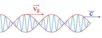
vitesse de groupe : v g = d ω d k v_{g}=\frac{d\omega}{dk} v g = d k d ω
sin ( k x − ω t ) + sin ( k ′ x − ω ′ t ) = 2 sin ( k ′ + d k 2 x − ω + ω ′ 2 t ) ⏟ v ϕ ≈ ω k cos ( k ′ − k 2 x − ω ′ − ω 2 t ) ⏟ v g ≈ d ω d k \sin(kx-\omega t)+\sin(k'x-\omega't)=2\sin\underbrace{(\frac{k'+dk}{2}x-\frac{\omega+\omega'}{2}t)}_{v_{\phi}\approx\frac{\omega}{k}}\cos\underbrace{(\frac{k'-k}{2}x-\frac{\omega'-\omega}{2}t)}_{v_{g}\approx\frac{d\omega}{dk}} sin ( k x − ω t ) + sin ( k ′ x − ω ′ t ) = 2 sin v ϕ ≈ k ω ( 2 k ′ + d k x − 2 ω + ω ′ t ) cos v g ≈ d k d ω ( 2 k ′ − k x − 2 ω ′ − ω t ) Figure 6: vitesse de groupe
Figure 7: animation vitesse de groupe (vert) versus phase (rouge)
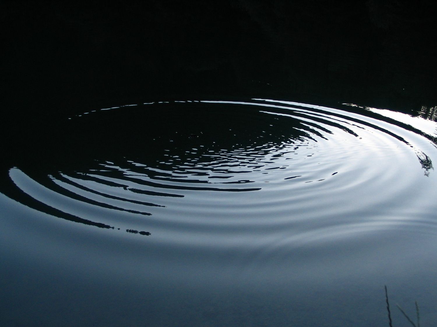
Figure 8: Ondes en eau peu profonde
en milieu peu profond L 0 ≫ h L_{0}\gg h L 0 ≫ h
déformation de la surface libre h ′ = A e k x − ω t h'=Ae^{kx-\omega t} h ′ = A e k x − ω t ω = k c 0 \omega=kc_{0} ω = k c 0
La célérité c 0 = g h c_{0}=\sqrt{gh} c 0 = g h k k k h h h
⟹ \Longrightarrow ⟹ v g = c 0 v_{g}=c_{0} v g = c 0 k k k
donc toutes les ondes se propagent à la même vitesse
⟹ \Longrightarrow ⟹ h h h
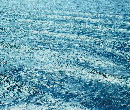
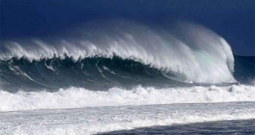
Modèle en eau profonde (océan) ¶ Figure 9: vagues sur l’océan
création des vagues par effet du vent puis propagation des vagues
attention milieu profond donc l’analyse précédente est non applicable
hypothèse :
pas d’effet du fond (h 0 h_{0} h 0 τ w \tau_{w} τ w ⇝ \leadsto ⇝
écoulement potentiel (irrotationnel)
U → = g r a d → ϕ \overrightarrow{U}=\overrightarrow{grad}\phi U = g r a d ϕ
h ′ ( x , y , t ) h'(x,y,t) h ′ ( x , y , t )
hauteur d’eau h ( x , y , t ) = h 0 + h ′ ( x , y , t ) h(x,y,t)=h_{0}+h'(x,y,t) h ( x , y , t ) = h 0 + h ′ ( x , y , t )
fond z = − h 0 z=-h_{0} z = − h 0
Si U → = g r a d → ϕ \overrightarrow{U}=\overrightarrow{grad}\phi U = g r a d ϕ
U → . ∇ U → = g r a d → ( 1 2 U 2 ) − U → ∧ r o t → U → = g r a d → ( 1 2 ( g r a d → ϕ ) 2 ) \overrightarrow{U}.\nabla\overrightarrow{U}=\overrightarrow{grad}(\frac{1}{2}U^{2})-\overrightarrow{U}\wedge\overrightarrow{rot}\,\overrightarrow{U}=\overrightarrow{grad}(\frac{1}{2}\left(\overrightarrow{grad}\phi\right)^{2}) U .∇ U = g r a d ( 2 1 U 2 ) − U ∧ ro t U = g r a d ( 2 1 ( g r a d ϕ ) 2 ) Le système d’équations s’écrit alors:
Δ Φ = 0 g r a d → ( ρ ∂ Φ ∂ t + ρ 2 ( g r a d → ϕ ) 2 + p + ρ g z ) = 0 \begin{aligned}
\Delta\Phi & =0\\
\overrightarrow{grad}\left(\rho\frac{\partial\Phi}{\partial t}+\frac{\rho}{2}\left(\overrightarrow{grad}\phi\right)^{2}+p+\rho gz\right) & =0\end{aligned} ΔΦ g r a d ( ρ ∂ t ∂ Φ + 2 ρ ( g r a d ϕ ) 2 + p + ρ g z ) = 0 = 0 On choisit d’écrire la pression sous la forme
p ( x , y , z , t ) = p 0 − ρ g z − ρ ∂ Φ ∂ t − ρ 2 ( g r a d → ϕ ) 2 p(x,y,z,t)=p_{0}-\rho gz-\rho\frac{\partial\Phi}{\partial t}-\frac{\rho}{2}\left(\overrightarrow{grad}\phi\right)^{2} p ( x , y , z , t ) = p 0 − ρ g z − ρ ∂ t ∂ Φ − 2 ρ ( g r a d ϕ ) 2 avec les conditions suivantes:
cdt limite au fond en z = − h 0 z=-h_{0} z = − h 0 U z = 0 Uz=0 U z = 0 ∂ Φ ∂ z = 0 \frac{\partial\Phi}{\partial z}=0 ∂ z ∂ Φ = 0
cdt limite à la surface libre en z = h ′ ( x , y , t ) z=h'(x,y,t) z = h ′ ( x , y , t ) V z = D h D t V_{z}=\frac{Dh}{Dt} V z = D t D h p = p 0 p=p_{0} p = p 0
Le système d’équations s’écrit alors:
∂ h ∂ t + ∂ h ∂ x ∂ Φ ∂ x + ∂ h ∂ y ∂ Φ ∂ y − ∂ Φ ∂ z = 0 ∂ Φ ∂ t + 1 2 ( g r a d → ϕ ) 2 = − g h ′ \begin{align*}
\frac{\partial h}{\partial t}+\frac{\partial h}{\partial x}\frac{\partial\Phi}{\partial x}+\frac{\partial h}{\partial y}\frac{\partial\Phi}{\partial y}-\frac{\partial\Phi}{\partial z}&=0\\
\frac{\partial\Phi}{\partial t}+\frac{1}{2}\left(\overrightarrow{grad}\phi\right)^{2}&= -gh'\\
\end{align*} ∂ t ∂ h + ∂ x ∂ h ∂ x ∂ Φ + ∂ y ∂ h ∂ y ∂ Φ − ∂ z ∂ Φ ∂ t ∂ Φ + 2 1 ( g r a d ϕ ) 2 = 0 = − g h ′ Ondes de surface en eau profonde ¶ Pour de petits mouvements h ′ ( x , t ) ≪ 1 h'(x,t)\ll1 h ′ ( x , t ) ≪ 1
ϕ ( x , z , t ) = A ( z ) e i k ( x − c t ) \phi(x,z,t)=A(z)e^{i\,k(x-ct)} ϕ ( x , z , t ) = A ( z ) e i k ( x − c t ) solution de l’équation:
Δ Φ = d 2 A d z 2 − k 2 A = 0 \Delta\Phi=\frac{d^{2}A}{dz^{2}}-k^{2}A=0 ΔΦ = d z 2 d 2 A − k 2 A = 0 La solution est de la forme
A ( z ) = A 0 c o s h ( k ( z + h 0 ) ) A(z)=A_{0}cosh(k(z+h_{0})) A ( z ) = A 0 cos h ( k ( z + h 0 )) qui vérifie la cdt ∂ Φ ∂ z = 0 \frac{\partial\Phi}{\partial z}=0 ∂ z ∂ Φ = 0 z = − h 0 z=-h_{0} z = − h 0
Cette solution vérifie les cdts (linéarisées) sur la surface libre:
z = h ′ avec h 0 + h ′ ≈ h 0 z=h' \mbox{ avec } h_{0}+h'\approx h_{0} z = h ′ avec h 0 + h ′ ≈ h 0
En notant c c c
∂ Φ ( x , h , t ) ∂ t = − g h ′ ⟹ h ′ = i k c g A 0 s i n h ( k h 0 ) e i k ( x − c t ) \frac{\partial\Phi(x,h,t)}{\partial t}=-gh'\Longrightarrow h'= i\frac{kc}{g}A_{0}sinh(kh_{0})e^{i\,k(x-ct)} ∂ t ∂ Φ ( x , h , t ) = − g h ′ ⟹ h ′ = i g k c A 0 s inh ( k h 0 ) e i k ( x − c t ) ∂ h ′ ∂ t = ∂ Φ ( x , h , t ) ∂ z = 0 ⟹ k 2 c 2 g A 0 c o s h ( k h 0 ) e i k ( x − c t ) = k A 0 s i n h ( k h 0 ) e i k ( x − c t ) \frac{\partial h'}{\partial t}=\frac{\partial\Phi(x,h,t)}{\partial z}=0\Longrightarrow\frac{k^{2}c^{2}}{g}A_{0}cosh(kh_{0})e^{i\,k(x-ct)}=kA_{0}sinh(kh_{0})e^{i\,k(x-ct)} ∂ t ∂ h ′ = ∂ z ∂ Φ ( x , h , t ) = 0 ⟹ g k 2 c 2 A 0 cos h ( k h 0 ) e i k ( x − c t ) = k A 0 s inh ( k h 0 ) e i k ( x − c t ) d’où la relation sur la célérité:
c 2 = g k tanh ( k h 0 ) soit ω 2 = k 2 c 2 = g k tanh ( k h 0 ) c^{2}=\frac{g}{k}\tanh(kh_{0}) \mbox{ soit }
\omega^{2}=k^{2}c^{2}=gk\tanh(kh_{0}) c 2 = k g tanh ( k h 0 ) soit ω 2 = k 2 c 2 = g k tanh ( k h 0 ) v g = d ω d k = 1 2 g k ≠ c = g k ∼ g λ avec λ = 2 π k v_{g}=\frac{d\omega}{dk}=\frac{1}{2}\sqrt{\frac{g}{k}}\neq c=\sqrt{\frac{g}{k}}\sim\sqrt{g\lambda}\,\mbox{ avec }\lambda=\frac{2\pi}{k} v g = d k d ω = 2 1 k g = c = k g ∼ g λ avec λ = k 2 π v g = c ∼ g h 0 v_{g}=c\sim\sqrt{gh_{0}} v g = c ∼ g h 0 Les paramètres pour les ondes en eau profonde sont :
Onde simple :
h ′ ( x , t ) = A sin ( k x − ω t + ϕ ) = A e i k ( x − c t ) + c c h'(x,t)=A\sin(kx-\omega t+\phi)=Ae^{i\,k(x-ct)}+cc h ′ ( x , t ) = A sin ( k x − ω t + ϕ ) = A e i k ( x − c t ) + cc
nombre d’onde k = 2 π λ k=\frac{2\pi}{\lambda} k = λ 2 π λ \lambda λ
pulsation ω = 2 π T = 2 π f \omega=\frac{2\pi}{T}=2\pi f ω = T 2 π = 2 π f T T T f f f
vitesse de phase (célérité): v ϕ = ω k = c v_{\phi}=\frac{\omega}{k}=c v ϕ = k ω = c
vitesse de groupe : v g = d ω d k v_{g}=\frac{d\omega}{dk} v g = d k d ω
sin ( k x − ω t ) + sin ( k ′ x − ω ′ t ) = 2 sin ( k ′ + d k 2 x − ω + ω ′ 2 t ) ⏟ v ϕ ≈ ω k cos ( k ′ − k 2 x − ω ′ − ω 2 t ) ⏟ v g ≈ d ω d k \sin(kx-\omega t)+\sin(k'x-\omega't)=2\sin\underbrace{(\frac{k'+dk}{2}x-\frac{\omega+\omega'}{2}t)}_{v_{\phi}\approx\frac{\omega}{k}}\cos\underbrace{(\frac{k'-k}{2}x-\frac{\omega'-\omega}{2}t)}_{v_{g}\approx\frac{d\omega}{dk}} sin ( k x − ω t ) + sin ( k ′ x − ω ′ t ) = 2 sin v ϕ ≈ k ω ( 2 k ′ + d k x − 2 ω + ω ′ t ) cos v g ≈ d k d ω ( 2 k ′ − k x − 2 ω ′ − ω t ) Figure 10: vitesse de groupe (vert) et de phase (rouge)
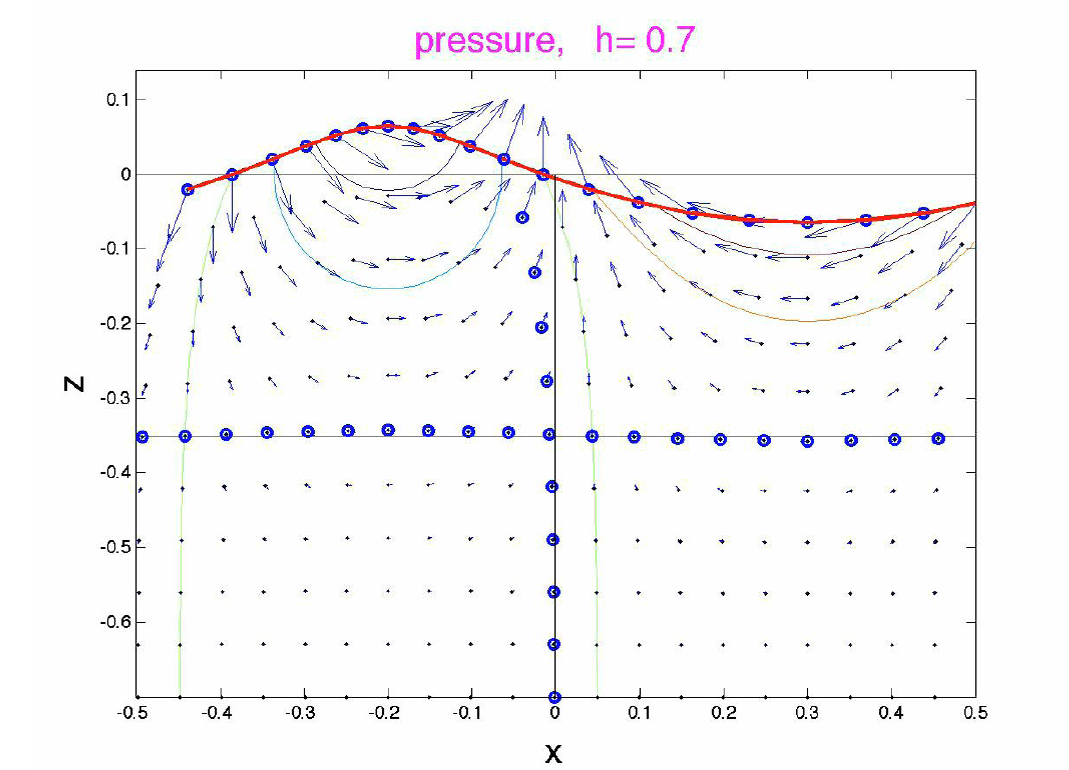
U = i k A 0 c o s h ( k ( z + h 0 ) ) e i k ( x − c t ) et W = k A 0 s i n h ( k ( z + h 0 ) ) e i k ( x − c t ) U=i\,kA_{0}cosh(k(z+h_{0}))e^{i\,k(x-ct)}\mbox{ et }W=kA_{0}sinh(k(z+h_{0}))e^{\bm{i}k(x-ct)} U = i k A 0 cos h ( k ( z + h 0 )) e i k ( x − c t ) et W = k A 0 s inh ( k ( z + h 0 )) e i k ( x − c t )
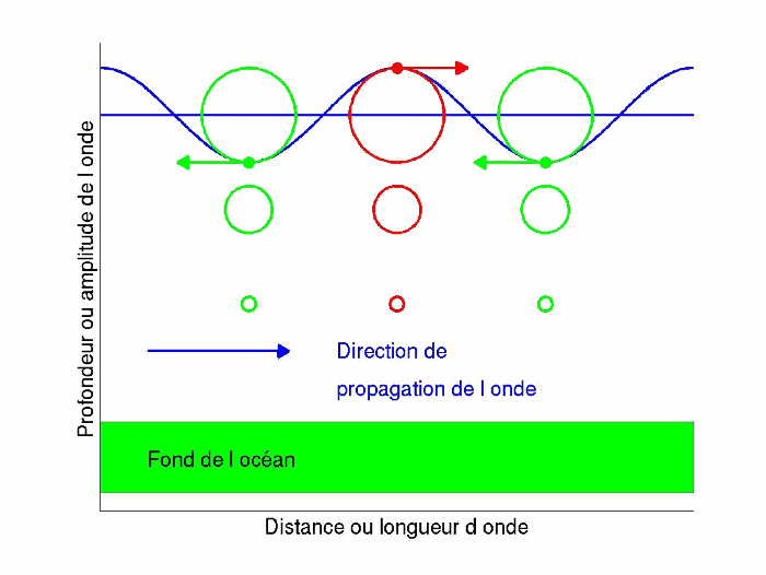
Figure 11: Ondes de surface
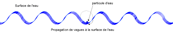
Figure 12: Propagation de vagues
Figure 13: animation de la propagation de vagues
Figure 14: houle
Figure 15: déferlement de vague
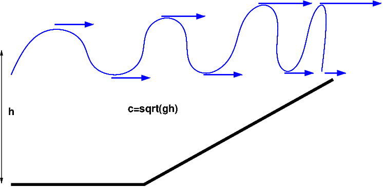
Près des cotes c ≈ g h c\approx\sqrt{gh} c ≈ g h h → 0 h\rightarrow0 h → 0 c ↗ c\nearrow c ↗
Figure 16: principe du déferlement de vague
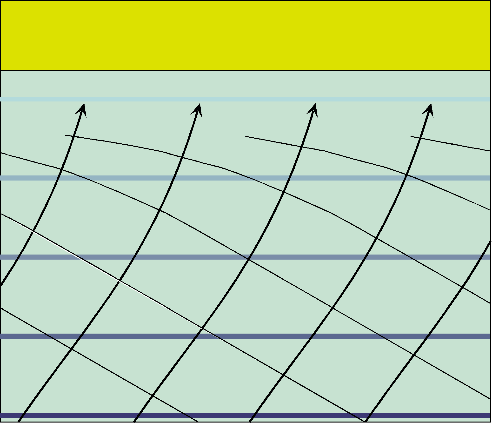
Quand la direction des houles est oblique par rapport à la côte, donc
aux isobathes (lignes d’égale profondeur), la vitesse de propagation de
la houle (c c c
Figure 17: houle sur la cote: en noir crêtes de houle, en bleu, isobathes
Le déferlement survient lorsque la houle arrive près de la côte
(phénomène de réfraction)Bonnefille, 1976
la vitesse de propagation c c c U U U
nombre caractéristique M = U / c M=U/c M = U / c
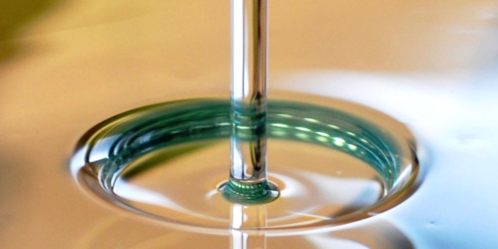
phénoménes de ressaut hydraulique (analogue au choc) si M > 1 M>1 M > 1
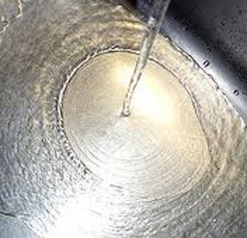
Figure 18: ressaut hydraulique
type d’ écoulement suivant le nombre de Froude F r = U 0 g h 0 Fr=\frac{U_{0}}{\sqrt{gh_{0}}} F r = g h 0 U 0
ressaut : passage torrentiel à fluvial (avec dissipation d’énergie)
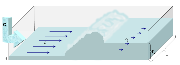
Figure 19: expérience de ressaut
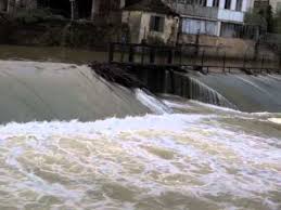
accélération du fluide en 2 (sur le barrage) > > >
transition vers régime fluviale en 4 < < <
Bernoulli sur la surface libre
E = g h + 1 2 u 2 = c s t e E=gh+\frac{1}{2}u^{2}=cste E = g h + 2 1 u 2 = cs t e Bilan masse
Q = h u = c s t e Q=hu=cste Q = h u = cs t e comparaison de u u u g h 0 \sqrt{gh_{0}} g h 0
Figure 20: ressaut hydraulique
Figure 21: ressaut hydraulique
Figure 22: sillage d’un navire
Soliton = onde solitaire qui se propage dans les milieux non linéaires
et dispersifs avec une énergie localisée dans l’espace (stable)
Figure 23: Mascaret
Figure 24: Tsunami
Bonnefille, R. (1976). Cours d’hydraulique maritime . Masson.