
- jeu. 20 juin 2019
- Cours
- #ipython jupyter
Table des matières
- 1 Etude d’un bras de robot 2D
- 2 Simulation géométrique
- 3 Cinématique inverse
- 4 Etude statique du bras de robot
- 5 Mouvement quasi-statique
- 6 Cinématique
- 7 Calcul des accélérations
- 8 Etude Dynamique
- 9 Contrôle de la position : choix des couples $C$
Etude et contrôle d’un bras de robot 2D
Modélisation sous python avec sympy mechanics
Marc BUFFAT, dpt mécanique, Université Claude Bernard Lyon 1
Mise à disposition selon les termes de la Licence Creative Commons
Attribution - Pas d’Utilisation Commerciale - Partage dans les Mêmes Conditions 2.0 France.
%matplotlib inline
%autosave 300
import numpy as np
import scipy as sp
import sympy as sp
import matplotlib.pyplot as plt
from matplotlib import rcParams
rcParams['font.family'] = 'serif'
rcParams['font.size'] = 14
from IPython.core.display import HTML
from IPython.display import display,Image
from matplotlib import animation
Some Tex macros & lib $$\newcommand{\dt}[1] {\frac{d{#1}}{dt}}$$ $$\newcommand{\bm}[1] {{\mathbf #1}}$$
from sympy.physics.vector import init_vprinting
init_vprinting(use_latex='mathjax', pretty_print=False)
Etude d’un bras de robot 2D
Objectifs
En utilisant un modèle mécanique simplifié d’un bras de robot à 2 degrés de liberté, on veut déterminer les commandes mécaniques pour positionner le bras de robot.
outils:
- utilisation du module sympy de calcul symbolique sous Python
- utilistion de la bibliothéque Classical Mechanics
analyse mécanique: symbolique + numérique
- analyse du mouvement, trajectoire (changement de repère)
- cinématique inverse
- analyse statique avec PF de la statique (avec le sforces de liaison) et et la formulation de Lagrange
- controle en quasi-statique
- analyse cinematique (calcul vitesse, torseur, changement de repère)
- analyse dynamique (calcul quantité de mouvement, moment cinétique, énergie)
- formulation de lagrange
- détermination de la commande du robot (par découplage + feedback)
- comparaison avec l’analyse quasi-statique
Système mécanique à 2 DDL
système mécanique à 2 DDL: $\theta_1$ et $\theta_2$
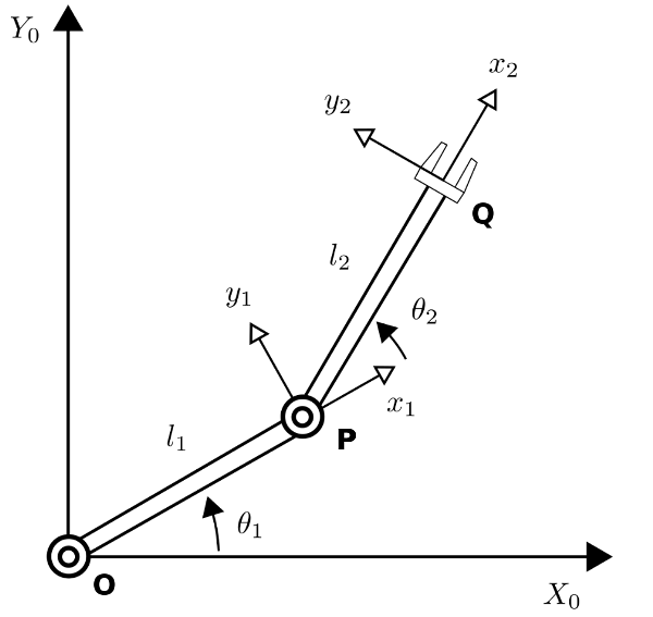
Modélisation avec sympy
- définition des paramêtres du problème et des DDL
- définition des points et des repéres
- définition de la position (dans les bons repères)
from sympy.physics.mechanics import dynamicsymbols, Point, ReferenceFrame
print("Définition des paramêtres (sous forme de symbol)")
l1, l2 = sp.symbols('l1 l2')
print("Parametres: ",l1,l2)
l1,l2
print("Définition des DDL, variables fonction du temps")
theta1, theta2 = dynamicsymbols('theta1 theta2')
print("DDL: ",theta1,theta2)
theta1,theta2
RO = ReferenceFrame('R_O')
RP = ReferenceFrame('R_P')
RQ = ReferenceFrame('R_Q')
- Définition de l’orientation des repères (rotation / Oz perpendiculaire au plan) / au repère fixe $R_O$
RP.orient(RO, 'Axis', [theta1, RO.z])
RQ.orient(RP, 'Axis', [theta2, RO.z])
- Matrice de rotation (3x3) pour passage du repere de base au repère de la main
T02 = RO.dcm(RQ)
T02.simplify()
Points
- Définition du point de référence $O$ et des 2 Points $P$ et $Q$ du robot
O = Point('O')
P = Point('P')
Q = Point('Q')
P.set_pos(O, l1 * RP.x)
Q.set_pos(P, l2 * RQ.x)
position de $Q$ dans le repère de base
Q.pos_from(O)
- dans le repère fixe $R_O$
qxy = (Q.pos_from(O).express(RO)).simplify()
qxy
composantes de $Q$ suivant x et y dans le repère $R_O$
qx=qxy.dot(RO.x)
qx
qy=qxy.dot(RO.y)
qy
idem pour le point $P$
pxy = (P.pos_from(O).express(RO)).simplify()
pxy
composante de $Q$ dans $R_O$
px = pxy.dot(RO.x)
py = pxy.dot(RO.y)
Simulation géométrique
conversion des formules analytiques en fonction python (numérique) avec lambdify
- fonction Qx,Qy calculant les coordonnées de $Q$ dans $R_O$
- fonction Px,Py calculant les coordonnées de $P$ dans $R_O$
les paramêtres sont les symbols intervenant dans les formules
Qx = sp.lambdify((l1, l2, theta1, theta2), qx, 'numpy')
Qy = sp.lambdify((l1, l2, theta1, theta2), qy, 'numpy')
Px = sp.lambdify((l1, theta1), px, 'numpy')
Py = sp.lambdify((l1, theta1), py, 'numpy')
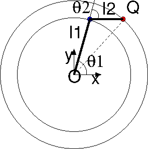
application numérique
calcul de la position du robot pour différentes valeurs de $\theta_1$ et $\theta_2$
- calcul des valeurs numériques
- choix des valeurs des paramétres
# nbre de valeurs de theta
Np=100
# longueur du bras en m
L1 = 0.5
L2 = 0.5
# variation des angles
theta1s = np.linspace(0, 2*np.pi,Np)
theta2s = np.linspace(0, 2*np.pi,Np)
# calcul de la positions fct angle
QX = np.array(Qx(L1, L2, theta1s, theta2s))
QY = np.array(Qy(L1, L2, theta1s, theta2s))
PX = np.array(Px(L1,theta1s))
PY = np.array(Py(L1,theta1s))
tracer de position
fig, (ax1,ax2) = plt.subplots(1,2,figsize=(12,6))
ax1.plot(np.rad2deg(theta1s), QX, label = r'$Q_x$')
ax1.plot(np.rad2deg(theta1s), QY, label = r'$Q_y$')
ax1.set_xlabel(r'($\theta_1$, $\theta_2$) [deg]')
ax1.set_ylabel(r' position [m]')
ax1.set_title('Position du point Q')
ax1.legend()
ax1.grid()
ax2.plot(QX,QY,label='Q')
ax2.plot(PX,PY,label='P')
ax2.set_title("Trajectoire")
ax2.legend();

Animation de la trajectoire
Fig=plt.figure(figsize=(8,8))
ax = Fig.add_subplot(111, aspect='equal')
ax.set_axis_off()
ax.set_xlim((-1.2*(L1+L2),1.2*(L1+L2)))
ax.set_ylim((-1.2*(L1+L2),1.2*(L1+L2)))
ax.set_title('mouvement du bras de robot',fontsize=30)
fig.set_facecolor("#ffffff")
line1, = ax.plot([0.,L1], [0.,0.], 'o-b', lw=18 , markersize=25)
line2, = ax.plot([L1,L1+L2], [0.,0.], 'o-', lw=18 , markersize=25)
pt1    = ax.scatter([L1+L2+0.05],[0.],marker="$\in$",s=800,c="black",zorder=3)
def animate(i):
    global PX,PY,QX,QY
    line1.set_data([0.,PX[i]],[0.,PY[i]])
    line2.set_data([PX[i],QX[i]],[PY[i],QY[i]])
    pt1.set_offsets([QX[i]+0.05,QY[i]])
    return line1,line2,pt1
anim = animation.FuncAnimation(Fig, animate, np.arange(1, Np), interval=50, blit=True)

HTML(anim.to_html5_video())
Cinématique inverse
problème: Si on fixe la position $Q$ de l’extrémité du bras, comment positionner le bras ?
- quelles sont les 2 angles $\theta_1$ et $\theta_2$ associées à une position $Q (x_2,y_2)$ fixée?
- problèmes non-linéaires !
- pas de solutions uniques
- plusieurs solutions ou aucunes solutions
- choix entre les solutions
$\leadsto$ résolution de 2 équations (non linéaires) en $\theta_1$ et $\theta_2$
Equations non linéaires en $\theta_1$,$\theta_2$ fonction de la position $x_2,y_2$ fixée
x2,y2=sp.symbols('x2 y2')
sp.Eq(x2,qx)
sp.Eq(y2,qy)
Méthodes de résolution
- analytique / géométrique
- numérique (Newton, méthode de gradient, calcul Jacobien)
bibliothéque scipy.optimize.root
### Méthode analytique loi des cosinus (pythagore généralisé)
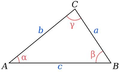
$$c^2 = a^2 + b^2 -2 a b \cos\gamma $$
solution analytique
$\theta_Q$ angle $<\widehat{\vec{OQ},\vec{Ox}}>$ $$ \cos\theta_Q = \frac{x_2}{\sqrt{x_2^2+y_2^2}}$$
$$\cos{(\theta_1 - \theta_Q)} = \frac{l_1^2 + x_2^2 + y_2^2 - l_2^2}{2 l_1 \sqrt{x_2^2+y_2^2}}$$$$\cos{(\theta_2 + \pi)} = \frac{l_1^2 + l_2^2 - (x_2^2+y_2^2)}{2 l_1 l_2}$$calcul de la solution analytique
# L1 et L2 définit précédemment
def cinematique_inv(x2,y2):
    '''calcul les angles theta1,theta2 du bras en fct de position fixée x2,y2'''
    global L1,L2
    L = np.sqrt(x2**2+y2**2)
    thetap = np.arccos(x2/L)
    theta1 = np.arccos((L1**2 + L**2  - L2**2)/(2*L1*L)) + thetap
    theta2 = np.arccos((L1**2 + L2**2 - L**2) /(2*L1*L2)) - np.pi
    return theta1,theta2
# calcul de la solution fonction d'un choix de position X,Y
# test validation
X, Y = np.sqrt(2)/2.0001*(L1+L2),np.sqrt(2)/2.0100*(L1+L2)
# cas 1
X, Y = (L1+L2)/1.5,L2/1.2
# cas 2 pble !!!
#X, Y = -(L1+L2)/2.,L2/3
# solution
Theta1p,Theta2p = cinematique_inv(X,Y)
X1, Y1 = Px(L1,Theta1p), Py(L1,Theta1p)
X2, Y2 = Qx(L1,L2,Theta1p,Theta2p), Qy(L1,L2,Theta1p,Theta2p)
print("Solution pour x2:{:6.2f}={:6.2f} y2:{:6.2f}={:6.2f} angles theta1={:5.3f}rd ({:6.2f}°) theta2={:5.3f} ({:6.2f}°)"
      .format(X,X2,Y,Y2,Theta1p,np.rad2deg(Theta1p),Theta2p,np.rad2deg(Theta2p)))
plt.figure()
plt.plot([0.,X1],[0.,Y1],'o-b',markersize=25,lw=18)
plt.plot([X1,X2],[Y1,Y2],'o-',markersize=25,lw=18)
plt.scatter([X+0.05],[Y],marker="$\in$",s=800,c="black",zorder=3)
plt.axis('equal')
plt.title("Position du robot");

Animation cinématique
Np = 50
theta1s = np.linspace(0, Theta1p,Np)
theta2s = np.linspace(0, Theta2p,Np)
# positions fct angle
QX = np.array(Qx(L1, L2, theta1s, theta2s))
QY = np.array(Qy(L1, L2, theta1s, theta2s))
PX = np.array(Px(L1,theta1s))
PY = np.array(Py(L1,theta1s))
anim = animation.FuncAnimation(Fig, animate, np.arange(1, Np), interval=40, blit=True)
HTML(anim.to_html5_video())
calcul solution numérique
- calcul numérique de la solution (racine ou root en anglais) d’un système d’équation $$\vec{F}(\vec{X^*})=\vec{0}$$
méthode itérative de Newton
calcul d’une suite $\vec{X^k}$ tq: $\vec{X^k} \ \rightarrow \ \vec{X^*}$
- DL de $\vec{F}(\vec{X^*})$ au voisinage de $\vec{X^k}$ à l’ordre 1 $$ \vec{F}(\vec{X^*}) = \vec{F}(\vec{X}^k) + \frac{\partial \vec{F}}{\partial \vec{X}} (\vec{X^*} - \vec{X^k}) $$
- méthode itérative $$ X^{k+1} = X^k + ( \nabla \vec{F^k} )^{-1} \vec{F}(\vec{X^k}) \mbox{ avec } \nabla \vec{F^k}=\frac{\partial \vec{F^k}}{\partial \vec{X}} $$
- calcul du jacobien exacte ou numérique
- convergence locale (importance point de départ $\vec{X^0}$)!!!
Equations $\vec{F}(\vec{X})=\vec{0}$ avec $\vec{X}=[\theta1,\theta2]$
sp.Eq(qx - x2,0)
sp.Eq(qy - y2,0)
Définition de la fonction F
from scipy.optimize import root
# recherche racine F(theta)=0 (X position voulue du bras)
def func(theta):
    '''calcul l'ecart F(theta)-X de position en fonction de theta=[theta1,theta2]'''
    global L1,L2,X,Y
    dx2 = Qx(L1, L2, theta[0], theta[1]) - X
    dy2 = Qy(L1, L2, theta[0], theta[1]) - Y
    return [dx2,dy2]
# choix du point de depart
sol = root(func,[0.,0.])
# autre choix
#sol = root(func,[np.pi/2,np.pi/2])
print(sol)
print("\nComparaison avec la solution analytique {:6.3f}={:6.3f} et {:6.3f}={:6.3f}".format(sol.x[0],Theta1p,sol.x[1],Theta2p))
# tracer de la position calculée
X1,Y1 = Px(L1,sol.x[0]), Py(L1,sol.x[0])
X2,Y2 = Qx(L1,L2,sol.x[0],sol.x[1]), Qy(L1,L2,sol.x[0],sol.x[1])
plt.figure()
plt.plot([0.,X1],[0.,Y1],'o-b',markersize=25,lw=18)
plt.plot([X1,X2],[Y1,Y2],'o-' ,markersize=25,lw=18)
plt.scatter([X+0.05],[Y],marker="$\in$",s=800,c="black",zorder=3)
plt.axis('equal')
plt.title("Position du robot");
Etude statique du bras de robot
solide en équilibre statique $\equiv$ la somme des forces appliquées et la somme des moments sont nulles
Pour le bras de robot:
- 2 solides indéformables: les 2 tiges OP et PQ
- une liaison pivot parfaite (sans frottement) en O et P
- force extérieur= gravité
- les 2 tiges OP et OQ ont chacune une masse $m_1$ et $m_2$ et un centre de gravité $G_1$ $G_2$ $$\vec{P_1}= - m_1 g \vec{R_O}_y \mbox{ et } \vec{P_2}= - m_2 g \vec{R_O}_y$$
- on suppose que le bras porte une masse $m$ à son extrémité $Q$ $$\vec{P_Q}= - m g \vec{R_O}_y$$
on applique des couples $C_1$ et $C_2$ (à l’aide de moteurs) en $O$ et $P$ pour imposer les angles $\theta_1$ et $\theta_2$
définition des paramêtres
C1,C2,m,m1,m2,g = sp.symbols('C1 C2 m m_1 m_2 g')
# centre de gravité
G1 = Point('G1')
G1.set_pos(O,l1/2 * RP.x)
yg1=G1.pos_from(O).express(RO).dot(RO.y)
G2 = Point('G2')
G2.set_pos(P,l2/2 * RQ.x)
yg2=G2.pos_from(O).express(RO).dot(RO.y)
display(yg1,yg2)
Modélisation des efforts à l’aide de torseur
Torseur : force et moment (couple) en un point $A$: $$ (\mathcal{T})_A = < \vec{R}, \vec{C_A} > $$ Calcul des torseurs et réduction en $P$:
- torseurs poids des tiges en $G_1$ et $G_2$
$$ (\mathcal{Tg_1})_{G_1} = <\vec{P_1},\vec{0}>$$
$$ (\mathcal{Tg_2})_{G_2} = <\vec{P_2},\vec{0}>$$
- réductions en $P$ $$ (\mathcal{Tg_1})_{P} = <\vec{P_1},\vec{P_1}\wedge{G_1P}>$$ $$ (\mathcal{Tg_2})_{P} = <\vec{P_2},\vec{P_2}\wedge{G_2P}>$$
- torseur poids en $Q$
$$ (\mathcal{Tg})_Q = <\vec{P_g},\vec{0}>$$
- torseur en $P$ $$ (\mathcal{Tg})_P = <\vec{P_g},\vec{P_g}\wedge\vec{QP}>$$
- liaison pivot en $P$:
- action de $OP$ sur $PQ$ $$ (\mathcal{T_{12}})_P = <\vec{R_{12}},\vec{0}>$$
- action de $PQ$ sur $OP$ $$ (\mathcal{T_{21}})_P = -(\mathcal{T_{12}})_P$$
- couple en $P$
- couple en $P$ exercé sur $PQ$: $C_2$ $$ (\mathcal{T_{\theta_2}})_P = <\vec{0},\vec{C_2}>$$
- couple en $P$ exercé sur $OP$: $-C_2$
- liaison pivot en O: action sur $OP$
$$ (\mathcal{T_{1}})_O = <\vec{R_{1}},\vec{0}>$$
- torseur en $P$ $$ (\mathcal{T_{1}})_P = <\vec{R_{1}},\vec{R_1}\wedge\vec{OP}>$$
- $C_1$ couple en $O$
$$ (\mathcal{T_{\theta_1}})_O = <\vec{0},\vec{C_1}>$$
- torseur en $P$ $$ (\mathcal{T_{\theta_1}})_P = <\vec{0},\vec{C_1}>$$
Bilan des forces
2 solides $OP$ et $PQ$
bilan des forces sur la tige $OP$ $$ (\mathcal{T_{\theta_1}})_P - (\mathcal{T_{\theta_2}})_P + (\mathcal{T_{1}})_P + (\mathcal{T_{21}})_P + (\mathcal{Tg_{1}})_P = (0)$$
bilan des forces sur la tige $PQ$ $$ (\mathcal{T_{\theta_2}})_P + (\mathcal{T_{12}})_P + (\mathcal{Tg})_P + (\mathcal{Tg_{2}})_P= (0) $$
4 inconnues pour 4 relations:
- 2 inconnues liaisons $\vec{R_1}$ et $\vec{R_{12}}$
- 2 couples $\vec{C_1}$ et $\vec{C_2}$
Solution
- forces de liaison $$ \vec{R_1} - \vec{R_{12}}= -\vec{Pg_{1}} $$ $$ \vec{R_{12}} = -\vec{Pg}-\vec{Pg_2} $$
couples en P $$ \vec{C_1} - \vec{C_2} = -\vec{R_1}\wedge\vec{OP} -\vec{Pg_1}\wedge\vec{G_1P} $$ $$ \vec{C_2} = -\vec{Pg}\wedge\vec{QP} -\vec{Pg_2}\wedge\vec{G_2P}$$
solution $$ \vec{R_{12}} = -\vec{Pg}-\vec{Pg_2} $$ $$ \vec{R_1} = -\vec{Pg}-\vec{Pg_2}-\vec{Pg_{1}}$$ $$ \vec{C2} = -\vec{Pg}\wedge\vec{QP} -\vec{Pg_2}\wedge\vec{G_2P}$$ $$ \vec{C1} = \vec{C2} -\vec{R_1}\wedge\vec{OP} -\vec{Pg_1}\wedge\vec{G_1P} $$
Formulation travaux virtuels
- Calcul du travail des forces extérieurs et des couples $$ \delta W = \sum \vec{F_i}.\vec{\delta x_i} + \sum \vec{C_j} \vec{\delta \theta_j} $$
- Equilibre statique $\delta W$ est nul pour tous les déplacements licites $\vec{\delta x_i}$ $\vec{\delta\theta_j}$
Avantage: élimination des liaisons car le travail des forces de liaison = 0 (liaison parfaite) #### calcul du travail $$ \delta W = C_1 \delta \theta_1 + C_2 \delta \theta_2 - m g \delta y_2 -m_1 g \delta y_{G1} -m_2 g \delta y_{G2} $$
calcul des déplacements verticaux licites $y_2$ de $Q$, $y_{G1}$ de $G_1$ et $y_{G2}$ de $G_2$ (fonction de $\theta_1$ et $\theta_2$).
d1,d2 = sp.symbols('delta_theta_1 delta_theta_2')
dy2 = sp.diff(qy,theta1)*d1 + sp.diff(qy,theta2)*d2
dyg1= sp.diff(yg1,theta1)*d1 + sp.diff(yg1,theta2)*d2
dyg2= sp.diff(yg2,theta1)*d1 + sp.diff(yg2,theta2)*d2
display(dy2,dyg1,dyg2)
dW = C1*d1 + C2*d2 - m*g*dy2 - m1*g*dyg1 - m2*g*dyg2
dW = sp.expand(dW)
dW
d’où les 2 relations pour que $dw=0$ $\forall \delta \theta_1$ et $\forall \delta \theta_2$
sp.Eq(sp.collect(dW,d2).coeff(d2,1).simplify())
sp.Eq(sp.collect(dW,d1).coeff(d1,1).simplify())
Formulation Lagrangienne
si une force $\vec{F}$ découle d’un potentiel $U$, $$ \vec{F} = -grad U $$ alors son travail s’écrit: $$\delta W = F \delta x = -\frac{\partial U}{\partial x} \delta x$$
- Equations de Lagrange en statique: coordonnées généralisées $q_i$
- définition du Lagrangien $$ L(q_i) = -U(q_i) $$
- bilan des travaux virtuels avec des forces généralisées $F_i$ $$ - \sum \frac{\partial L}{\partial q_i} \delta q_i = \sum F_i \delta q_i $$
- équations de Lagrange $$ -\frac{\partial L}{\partial q_i} = F_i $$
calcul lagrangien (potentiel de gravité)
L = -m*g*qy - m1*g*yg1 - m2*g*yg2
L
Equations de Lagrange
forces extérieurs $C_1$ et $C_2$
sp.Eq(-sp.diff(L,theta1).simplify(),C1)
sp.Eq(-sp.diff(L,theta2).simplify(),C2)
Mouvement quasi-statique
à chaque instant équilibre quasi-statique (mouvement lent)
- calcul des couples a appliquer pour arriver à une position fixée
- paramétres numériques
print("angles (position finale): ",Theta1p,Theta2p)
params = [(g,9.81), (m,10), (m1,1), (m2,1), (l1, L1), (l2, L2)]
params
funC1 = sp.lambdify([theta1,theta2],-sp.diff(L,theta1).subs(params))
funC2 = sp.lambdify([theta1,theta2],-sp.diff(L,theta2).subs(params))
THETA1 = np.linspace(np.pi/2,Theta1p,Np)
THETA2 = np.linspace(-np.pi,Theta2p,Np)
FC2 = funC2(THETA1,THETA2)
FC1 = funC1(THETA1,THETA2)
X1 = Px(L1,THETA1)
Y1 = Py(L1,THETA1)
X2 = Qx(L1,L2,THETA1,THETA2)
Y2 = Qy(L1,L2,THETA1,THETA2)
plt.figure(figsize=(12,6))
plt.subplot(1,2,1)
plt.plot(FC1,label="C1")
plt.plot(FC2,label="C2")
plt.legend()
plt.title('couples')
plt.subplot(1,2,2)
plt.plot(X1,Y1,label='P')
plt.plot(X2,Y2,label='Q')
plt.title('trajectoire')
plt.plot([0,X1[-1],X2[-1]],[0.,Y1[-1],Y2[-1]],'-ok',lw=10,markersize=25)
plt.legend()
plt.axis('equal');

O.set_vel(RO,0.)
P.v2pt_theory(O,RO,RP)
VP = P.vel(RO)
VP
calcul vitesse en $Q$
- vitesse de $Q$ qui est dans le meme solide que $P$ (repere $R_Q$)
- utilisation de la composition des vitesses $$ \vec{V_Q}|R_O = \vec{V_P}|R_O + \Omega_{R_Q} \wedge \vec{PQ} $$
Q.v2pt_theory(P,RO,RQ)
VQ = Q.vel(RO)
VQ
VQ.express(RO).simplify()
vérification de la composition des vitesses
- formule de composition des vitesses:
- solide $PQ\in R_Q$ et vitesse de rotation $\Omega_{R_Q}$ de $R_Q / R_O$: $$ \vec{V_Q}|R_O = \vec{V_P}|R_O + \Omega_{R_Q} \wedge \vec{PQ} $$
- calcul directe
WQ = RQ.ang_vel_in(RO)
WQ
PQ = Q.pos_from(P)
P.vel(RO) + WQ.cross(PQ)
Calcul des accélérations
calcul accélération de $P$
- utilisation composition des accélérations
- fonction a2pt_theory
- projection dans le repère fixe $R_O$
P.a2pt_theory(O,RO,RP)
GP = P.acc(RO)
GP
# projection dans le repere fixe R_O
GP.express(RO)
calcul accélération de $Q$
Q.a2pt_theory(P,RO,RQ)
GQ = Q.acc(RO)
GQ.simplify()
- projection dans $R_O$
GQ.express(RO).simplify()
vérification de la formule de composition des accélérations
formule de composition des accélérations ($P,Q \in R_Q$):
- solide $PQ\in R_Q$ et vitesse de rotation de $R_Q / R_O$: $\Omega_{R_Q}$ $$ \vec{\Gamma}_Q | R_O = \vec{\Gamma}_P| R_O + \frac{d}{dt}(\vec{\Omega}_{R_Q}) \wedge \vec{PQ} + \vec{\Omega}_{R_Q}\wedge\vec{\Omega}_{R_Q}\wedge\vec{PQ} $$
rotation WQ et accéleration angulaire AQ de $R_Q$ / $R_O$
# taux rotation et accelération angulaire
WQ = RQ.ang_vel_in(RO)
AQ = RQ.ang_acc_in(RO)
AQ
# calcul vecteur PQ
PQ = Q.pos_from(P)
P.acc(RO) + AQ.cross(PQ) + WQ.cross(WQ.cross(PQ))
Etude Dynamique
Principe fondamentale de la dynamique (PFD):
pour chaque solide indéformable:
- variation de la quantité de mouvement = somme des forces extérieures
- variation du moment cinétique en $A$ = somme des moments de sforces en $A$
$\equiv$ relation sur les torseurs:
- torseur dynamique = somme des torseurs des forces appliquées
Dynamique de la tige $OP$
la tige $OP$ est un solide (cylindre homogène):
- de longueur $l_1$ et de rayon $r_1$
- de masse $m_1$
- de centre de gravité $G_1$ tq $\vec{OG_1} = \frac{1}{2} \vec{OP}$
de matrice d’inertie en $G_1$ dans $R_P$
$$I_1(G_1,R_P) = \begin{pmatrix} I_{1,x} & 0 & 0 \ 0 & I_{1,y} & 0 \ 0 & 0 & I_{1,y} \end{pmatrix}$$
- avec $I_{1,x} = \frac{1}{2} m_1 r_1^2 $ et $I_{1,y} = \frac{1}{4} m_1 r_1^2 + \frac{1}{12} m_1 l_1^2$
# symbols et inertie
from sympy.physics.mechanics import inertia
I1x,I1y = sp.symbols('I_1x I_1y')
I1 = inertia(RP,I1x,I1y,I1y)
I1
# vitesse du centre de gravité G1
G1.v2pt_theory(O,RO,RP)
G1.pos_from(O), G1.vel(RO)
Quantité de mouvement et moment cinétique
from sympy.physics.mechanics import RigidBody
TigeOP = RigidBody('Tige_OP',G1,RP,m1,(I1,G1))
from sympy.physics.mechanics import linear_momentum, angular_momentum
linear_momentum(RO,TigeOP), angular_momentum(G1,RO,TigeOP)
Energie cinétique
from sympy.physics.mechanics import kinetic_energy, potential_energy
kinetic_energy(RO, TigeOP)
Energie potentielle
TigeOP.potential_energy = m1*g*G1.pos_from(O).dot(RO.y)
potential_energy(TigeOP)
dérivée quantité mouvement
m1*G1.acc(RO)
Dynamique de la tige $PA$
la tige $PQ$ est un solide (cylindre homogène):
- de longueur $l_2$ et de rayon $r_2$
- de masse $m_2$
- de centre de gravité $G_2$ tq $\vec{PG_2} = \frac{1}{2} \vec{PQ}$
de matrice d’inertie en $G_2$ dans $R_Q$ $$I_2(G_2,R_Q) = \begin{pmatrix} I_{2,x} & 0 & 0 \ 0 & I_{2,y} & 0 \ 0 & 0 & I_{2,y} \end{pmatrix}$$
- avec $I_{2,x} = \frac{1}{2} m_2 r_2^2 $ et $I_{2,y} = \frac{1}{4} m_2 r_2^2 + \frac{1}{12} m_2 l_2^2$
I2x,I2y,m = sp.symbols('I_2x I_2y m')
I2 = inertia(RQ,I2x,I2y,I2y)
# vitesse du centre de gravité
G2.v2pt_theory(P,RO,RQ)
quantité de mouvement et moment cinétique
TigePQ = RigidBody('Tige_PQ',G2,RQ,m2,(I2,G2))
linear_momentum(RO,TigePQ), angular_momentum(G2,RO,TigePQ)
énergie cinétique et potentielle
kinetic_energy(RO,TigePQ)
# on ajoute la masse M en Q
TigePQ.potential_energy = m2*g*G2.pos_from(O).dot(RO.y) + m*g*Q.pos_from(O).dot(RO.y)
potential_energy(TigePQ)
Energie cinétique du bras de robot
Energie $= \sum$ energies des solides
kinetic_energy(RO,TigeOP,TigePQ).simplify()
potential_energy(TigeOP,TigePQ).simplify()
Calcul du lagrangien
pour le bras de robot: $ L = T - U$
from sympy.physics.mechanics import Lagrangian, LagrangesMethod
L = Lagrangian(RO,TigeOP,TigePQ).simplify()
L
Equations de Lagrange
LM = LagrangesMethod(L,[theta1,theta2], forcelist = [(RP, (C1-C2)*RO.z),(RQ, C2*RO.z)], frame = RO)
eqs = LM.form_lagranges_equations()
display(sp.Eq(eqs[0].expand(),0))
display(sp.Eq(eqs[1].expand(),0))
forme matricielle
- DDL $\mathbf{q}=[\theta_1,\theta_2]$
- matrice d’inertie $M_q$
- vecteur des couples extérieures $\mathbf{C}=[C_1, C_2]$ $$ M_q \ddot{\mathbf{q}} = F(\mathbf{q},\dot{\mathbf{q}}) + \mathbf{C}$$
C=sp.Array([[C1],[C2]])
C
MQ=LM.mass_matrix
display(MQ)
FQ=LM.forcing-C
display(FQ)
Contrôle de la position : choix des couples $C$
On applique les couples $\mathbf{C}$ par une opération de découplage et feedback en fonction de $u$ $$ \mathbf{C} = M_q \mathbf{u} - F(\mathbf{q},\dot{\mathbf{q}})$$ ce qui conduit à un système d’EDO linéaires indépendantes ($u$ étant fixé) $$ M_q \ddot{\mathbf{q}} = M_q \mathbf{u} \mbox{ soit } \ddot{\mathbf{q}} = \mathbf{u} $$
définition de commande $u$
On veut positionner le robot avec des angles fixés $\mathbf{q}^d = [\theta_1^d, \theta_2^d]$
On applique donc une commande $\mathbf{u}$ proportionnelle dérivée (feedback): $$ \mathbf{u} = -k_p (\mathbf{q}-\mathbf{q}^d) - k_v \dot{\mathbf{q}} $$ L’équation du mouvement se réduit à : $$ \ddot{\mathbf{q}} + k_v \dot{\mathbf{q}} + k_p (\mathbf{q}-\mathbf{q}^d) = 0 $$
On choisit les constantes $k_p$ et $k_v$ de façon à être dans le régime critique, i.e. avoir un retour à la position le plus rapidement possible sans oscillation. Le discrimant de l’équation carcatéristique est alors nul $$ \Delta = k_v^2 - 4 k_p = 0 \mbox{ soit } k_p = k_v^2/4 $$
q = sp.Function('q')
t = sp.Symbol('t',positive=True)
kv = sp.symbols('k_v',positive=True)
qd,q0 = sp.symbols('q_d q_0')
eq = sp.Eq(sp.Derivative(q(t),t,t) + kv*sp.Derivative(q(t),t) + kv*kv/4*(q(t)-qd) , 0 )
eq
solq=sp.dsolve(eq, q(t), ics={q(0):q0, q(t).diff(t).subs(t,0):0})
qs=sp.Lambda(t,solq.rhs)
qs(t)
from sympy.plotting import plot
plot(qs(t).subs([(qd,0),(q0,1),(kv,10)]), (t,0,2), ylabel='q(t)',title='solution critique');

theta1d,theta10,theta2d,theta20 = sp.symbols('theta_1_d theta_1_0 theta_2_d theta_2_0')
theta1s=sp.Lambda(t,qs(t).subs([(qd,theta1d),(q0,theta10)]))
theta2s=sp.Lambda(t,qs(t).subs([(qd,theta2d),(q0,theta20)]))
theta1s(t),theta2s(t)
commandes $u_1(t)$ et $u_2(t)$
u1 = -kv*sp.diff(theta1s(t),t) + kv*kv/4*(theta1s(t)-theta1d)
u1s = sp.Lambda(t,u1.simplify())
display(u1s(t))
u2 = -kv*sp.diff(theta2s(t),t) + kv*kv/4*(theta2s(t)-theta2d)
u2s = sp.Lambda(t,u2.simplify())
display(u2s(t))
couples $C_1$ et $C_2$
connaissant $\theta$ et $u$, on calcul $C$ t.q.: $$ \mathbf{C} = M_q \mathbf{u} - F(\mathbf{q},\dot{\mathbf{q}})$$
display(MQ,FQ)
génération de code
- fonction lambdify
- valeurs numériques des paramêtres
# liste supplémentaire des parametres
params=[ (I1y, m1*(0.02**2/4. + l1**2/12.)), (I2y, m2*(0.02**2/4. + l2**2/12.))] + params
params
génération des fonctions
- calcul de $\theta$
- calcul de $\dot{\theta}$
- calcul du contrôle $u$
- calcul du couple $C$
# notation pour les dérivées premières
theta1p, theta2p = dynamicsymbols('theta1 theta2',level=1)
# fonctions python
Theta1s = sp.lambdify((t,theta10,theta1d,kv),theta1s(t))
Theta2s = sp.lambdify((t,theta20,theta2d,kv),theta2s(t))
dTheta1s = sp.lambdify((t,theta10,theta1d,kv),sp.diff(theta1s(t),t))
dTheta2s = sp.lambdify((t,theta20,theta2d,kv),sp.diff(theta2s(t),t))
U1s     = sp.lambdify((t,theta10,theta1d,kv),theta1s(t))
U2s     = sp.lambdify((t,theta20,theta2d,kv),theta2s(t))
MQs     = sp.lambdify((theta1,theta2,theta1p,theta2p),MQ.subs(params))
FQs     = sp.lambdify((theta1,theta2,theta1p,theta2p),FQ.subs(params))
Calcul du contrôle
valeur des parametres
- positions et vitesses initiales
- positions finales
- valeur de $k_v$
Theta10 = np.pi/2
Theta20 = -np.pi
Kv = 10.0
C
def Thetas(t):
    """solution a t"""
    return np.array([Theta1s(t,Theta10,Theta1p,Kv),Theta2s(t,Theta20,Theta2p,Kv)])
def dThetas(t):
    """dérivée de la solution a t"""
    return np.array([dTheta1s(t,Theta10,Theta1p,Kv),dTheta2s(t,Theta20,Theta2p,Kv)])
def Couples(T):
    C = np.zeros((2,T.size))
    for k,t in enumerate(T):
        theta1  = Theta1s(t,Theta10,Theta1p,Kv)
        dtheta1 = dTheta1s(t,Theta10,Theta1p,Kv)
        theta2  = Theta2s(t,Theta20,Theta2p,Kv)
        dtheta2 = dTheta2s(t,Theta20,Theta2p,Kv)
        U = np.array([U1s(t,Theta10,Theta1p,Kv),U2s(t,Theta20,Theta2p,Kv)])
        M = MQs(theta1,theta2,dtheta1,dtheta2)
        F = FQs(theta1,theta2,dtheta1,dtheta2)[:,0]
        C[:,k] = np.dot(M,U)-F
    return C
Solution de contrôle du bras en dynamique
- comparaison du contrôle dynamique du bras avec la solution quasi-statique
T = np.linspace(0,2.0,Np)
THETA = Thetas(T)
CC    = Couples(T)
X1 = Px(L1,THETA[0,:])
Y1 = Py(L1,THETA[0,:])
X2 = Qx(L1,L2,THETA[0,:],THETA[1,:])
Y2 = Qy(L1,L2,THETA[0,:],THETA[1,:])
plt.figure(figsize=(12,8))
plt.subplot(1,2,1)
plt.plot(X1,Y1,label='P')
plt.plot(X2,Y2,label='Q')
plt.title('trajectoire')
plt.plot([0,X1[-1],X2[-1]],[0.,Y1[-1],Y2[-1]],'-ok',lw=10,markersize=25)
plt.legend()
plt.axis('equal')
plt.subplot(1,2,2)
plt.plot(T,CC[0,:],label='C1')
plt.plot(T,CC[1,:],label='C2')
plt.plot(T,FC1,'--',label="C1 statique")
plt.plot(T,FC2,'--',label="C2 statique")
plt.legend()
plt.title("Commandes du bras");

comparaison du mouvement (modèle dynamique / modèle quasi-statique)
plt.figure(figsize=(12,6))
plt.subplot(1,2,1)
plt.plot(THETA1,label="statique")
plt.plot(THETA[0,:],label="dynamique")
plt.legend()
plt.title("trajectoire $\\theta_1$")
plt.subplot(1,2,2)
plt.plot(THETA2,label="statique")
plt.plot(THETA[1,:],label="dynamique")
plt.legend()
plt.title("trajectoire $\\theta_2$");

Np = 50
theta1s = THETA[0,:]
theta2s = THETA[1,:]
# positions fct angle
QX = np.array(Qx(L1, L2, theta1s, theta2s))
QY = np.array(Qy(L1, L2, theta1s, theta2s))
PX = np.array(Px(L1,theta1s))
PY = np.array(Py(L1,theta1s))
anim = animation.FuncAnimation(Fig, animate, np.arange(1, Np), interval=40, blit=True)
HTML(anim.to_html5_video())
FIN
print("Version (attention bug avec sympy 1.1)")
print("sympy version:",sp.__version__)