
- lun. 05 février 2018
- Cours
- #ipython jupyter
%matplotlib inline
%autosave 300
import numpy as np
import scipy as sp
import matplotlib.pyplot as plt
from matplotlib import rcParams
rcParams['font.family'] = 'serif'
rcParams['font.size'] = 14
from IPython.core.display import HTML
from IPython.display import display
from matplotlib import animation
css_file = 'style.css'
HTML(open(css_file, "r").read())
# edit metadata   "livereveal": { "scroll": true }
# https://damianavila.github.io/RISE/customize.html
Discrétisation des EDP hyperboliques (II)
Marc BUFFAT, dpt mécanique, Université Claude Bernard Lyon 1 \begin{equation*} \newcommand{Dx}{\Delta x} \newcommand{Dt}{\Delta t} \newcommand{imh}{{i-\frac{1}{2}}} \newcommand{iph}{{i+\frac{1}{2}}} \newcommand{im}{{i-1}} \newcommand{ip}{{i+1}} \newcommand{dx}[1]{\frac{\partial #1}{\partial x}} \newcommand{dt}[1]{\frac{\partial #1}{\partial t}} \end{equation*}
équation de conservation générale
$$ \dt{Q} + \dx{F(Q)} = 0 $$Schéma volumes finis
maillage volumes finis
approximation constante sur chaque élèment
intrégration sur un volume élèmentaire $[x_\imh, x_\iph]$ entre $t^n$ et $t^n+\Dt$
schéma semi-discret: $$ Q^{n+1} - Q^n = -\frac{\Dt}{\Dx} \left( F_\iph - F_\imh \right) $$
flux à l’interface $F_\iph$ $$ F_\iph = \frac{1}{\Dt} \int_{t^n}^{t^n+\Dt} F(Q_\iph,t) dt $$
Equation de Burgers
Equation de burgers:
$$ \dt{u} + u \dx{u} = 0 $$sous forme conservative:
$$ \dt{u} + \dx{f(u)} = 0 \mbox{ avec } f(u)=\frac{1}{2} u^2 $$centré : instable $$ F_{\iph} =\frac{1}{4} \left( {u^n_{i}}^2 +{u^n_{i+1}}^2 \right)$$
upwind :
$$ F_{\iph} = \frac{1}{2} {u^n_{i}}^2 \mbox{ si } u_i > 0 $$
$$ F_{\iph} = \frac{1}{2} {u^n_{i+1}}^2 \mbox{ si } u_i < 0 $$
schéma UPWIND
def Upwind(U0,cfl,n):
    '''calcul solution burgers avec schéma VF au bout de n iterations'''
    Un = U0.copy()
    for i in range(n):
        # flux et schéma avec u>0
        Fr = 0.5*Un[1:-1]**2
        Fl = 0.5*Un[0:-2]**2
        Un[1:-1] = Un[1:-1] - cfl*(Fr-Fl)
        # cdt neumann
        Un[0] = Un[1]
        Un[-1]= Un[-2]
    return Un.copy()
# simulation sur un maillage
def simulUpwind(m,CFL):
    '''m nbre de pts, CFL'''
    L = 2.0
    X = np.linspace(0,L,m)
    dx = L/(m-1)
    # maillage fictif (avec cellules fictives)
    XX = np.zeros(m+2)
    XX[1:-1] = X
    XX[0] = -X[1]
    XX[-1]= XX[-2]+X[1]
    # pas en temps
    dt = CFL*dx/1
    n=int(1.6/dt)
    tf=n*dt
    print("parametres: CFL=%5.2f m=%d tf=%5.2f"%(CFL,m,tf))
    # CI
    Ul = 1.0
    Ur = 0.2
    a = (Ul+Ur)/2.0
    U_0 = lambda x: (Ul-Ur)*(1-(x>0.5).astype(float))+Ur
    U0 = U_0(XX)
    Uf = U_0(XX-a*tf)
    # calcul solution
    plt.figure(figsize=(14,6))
    plt.plot(XX,U0)
    U = Upwind(U0,CFL,n)
    plt.plot(XX,U,label="upwind")
    plt.plot(XX,Uf,'--k',label="exact")
    plt.legend(loc=0)
    return
simulUpwind(m=101,CFL=0.2)

from ipywidgets import interact,fixed
import warnings
warnings.filterwarnings(action='ignore')
interact(simulUpwind,m=[21,51,101,201,501],CFL=fixed(0.2))
Modèle de traffic routier
modèle de Lighthill-Whitham-Richards (1955)
Soit $\rho(x,t)$ la densité de traffic (i.e. le nombre de voiture par unité de longueur) $$\mbox{ aucune voiture } = 0 \le \rho \le \rho_{max} = \mbox{par choc contre pare choc}$$
L’équation d’évolution de $\rho$ est une equation de conservation: $$ \frac{\partial \rho}{\partial t} + \frac{\partial F}{\partial x} = 0$$ où $F=\rho u$ est le flux de voiture ($u$ est la vitesse des voitures)
- la vitesse tends vers la vitesse max si la route est libre
- la vitesse tends vers zero en cas de bouchon
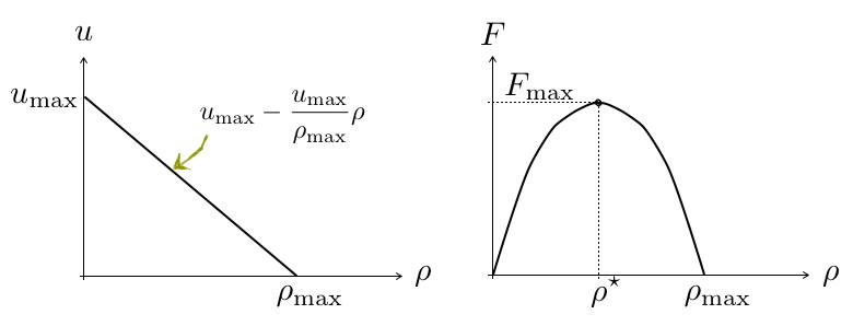
Un modèle simple suppose une dépendance linéaire decroissance de $u$ en fonction de $\rho$ $$ u(\rho) = u_{max} ( 1 - \frac{\rho}{\rho_{max}}) $$ d’ou un flux quadratique en $\rho$ $$ F = \rho u = \rho u_{max} ( 1 - \frac{\rho}{\rho_{max}}) $$
def flux(rho):
    global u_max,rho_max
    return rho*u_max*(1-rho/rho_max)
def vitesse(rho):
    global u_max
    return u_max*(1-rho/rho_max)
def trace(rho):
    global XX
    plt.figure(figsize=(12,6))
    plt.plot(XX,rho,lw=2)
    plt.title("densité de voiture")
    return
simulation de traffic lors du passage d’un feu au vert
On considère une route de longueur $L$ avec $u_{max}=1$ et $\rho_{max}=10$
A $t=0$ on a un feu rouge à $x=2$ et le feu passe au vert pour $t>0$
A l’instant initial, avant le feu, on suppose que le traffic décroit de $\rho_{max}$ vers zero et est nulle après le feu.
$$\rho(x,0) = \left\{ \begin{array}{cc}\rho_{max}\frac{x}{2} & 0 \leq x < 2\ 0 & 2 \leq x \leq 4 \ \end{array} \right.$$# maillage
L=6.0
rho_max=10.
u_max=1.0
# discretisation
nx=201
dx=L/(nx-1)
X = np.linspace(0,L,nx)
XX = np.zeros(nx+2)
XX[1:-1] = X
XX[0] = -dx
XX[-1]= XX[-2] + dx
def rho_init(rho_feu,XX):
""" champ initial """
global rho_max
rho=rho_feu*(XX/2.0)
rho=rho*(XX<=2.0).astype(int)
rho[0]=0.0
return rho
# condition initiale
rho_s=rho_max
rho0=rho_init(rho_s,XX)
trace(rho0)

schéma UPWIND
def Upwind(rho0,cfl,n):
global u_max,rho_max
'''calcul solution avec schéma VF au bout de n iterations'''
rho_n = rho0.copy()
for i in range(n):
F = flux(rho_n)
# schéma
rho_n[1:-1] = rho_n[1:-1] - cfl*(F[1:-1]-F[:-2])
# cdt neumann
rho_n[0] = rho_n[1]
rho_n[-1]= rho_n[-2]
return rho_n.copy()
# calcul
CFL=0.5
Nit=6
rho=rho0.copy()
plt.figure(figsize=(12,6))
plt.ylim([0,20])
plt.plot(XX,rho,lw=3)
for it in range(Nit):
rho=Upwind(rho,CFL,10)
plt.plot(XX,rho,lw=3)

analyse
divergence !!!
la vitesse de propagation n'est pas la bonne!!!
calcul du flux
$$ \frac{\partial \rho}{\partial t} + \frac{\partial F}{\partial x} = \frac{\partial \rho}{\partial t} + \frac{\partial F}{\partial \rho}\frac{\partial \rho}{\partial x} = 0$$pour le cas précédent $$\frac{\partial F}{\partial \rho} = u_{max} ( 1 - \frac{2\rho}{\rho_{max}}) $$ La vitesse de propagation $u_{max}( 1 - \frac{2\rho}{\rho_{max}})$ change de signe pour $\rho>\frac{\rho_{max}}{2}$
vérification
on modifie la CI pour avoir une propagation >0 .
$$\rho(x,0) = \left\{ \begin{array}{cc}\rho^*\frac{x}{2} & 0 \leq x < 2 \0 & 2 \leq x \leq 4 \ \end{array} \right.$$avec $\rho^* = \rho_{max}/2 $
CFL=0.5
Nit=6
rho_s=rho_max/2.
rho0=rho_init(rho_s,XX)
rho=rho0.copy()
plt.figure(figsize=(12,6))
plt.ylim([0,6])
plt.plot(XX,rho,lw=3)
for it in range(Nit):
rho=Upwind(rho,CFL,20)
plt.plot(XX,rho,lw=3)

Problème de Riemann
résolution d’un problème hyperbolique
$$ \dt{Q} + \dx{F(Q)} = 0 $$- schéma conservatif semi-discret: $$ Q^{n+1} - Q^n = -\frac{\Dt}{\Dx} \left( F_\iph - F_\imh \right) $$
- flux à l’interface $F_\iph$ $$ F_\iph = \frac{1}{\Dt} \int_{t^n}^{t^n+\Dt} F(Q_\iph,t) dt $$
- calcul du flux
- formulation conservative
- critère de décentrement n’est pas le signe de la vitesse
- le décentrement doit tenir compte de la vitesse de propagation des ondes
calcul de $F_\iph$
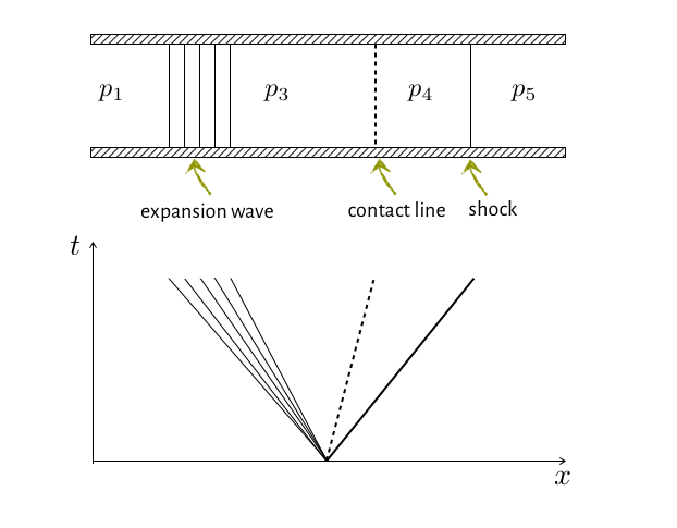
sur chaque interface $x_\iph$ on doit résoudre un problème du type tube à choc:
avec un état à gauche $Q^i$ et un état à droite $Q^{i+1}$
problème de Riemann : propagation d’ondes avec des célérités $\lambda_k$
problèmes de Riemann pour tout le maillage

solution = somme des solutions élèmentaires
conditions sur le problème de Riemann
solutions élémentaires n’inter-agissent pas entre elles
condition de stabilité de type CFL
$\lambda_k$ célérité des ondes = valeurs propes de la jacobienne des fluxs
$$ \lambda_k = v.p \left(\frac{\partial F}{\partial Q}\right)$$
relations de Rankine Hugoniot: propagation discontinuité entre 2 états $Q_L$ et $Q_R$
$$ (Q_R - Q_L) s = F(Q_R) - F(Q_L) $$ avec $s=\lambda_k$ célérité de la discontinuité
calcul du flux numérique $F_\iph$
schéma explicite centré: $$ F_\iph = \frac{1}{2} \left( F(Q^n_{i+1}) + F(Q^n_i)\right) $$ instable
schéma de Godounov (décentré)
- décentrement fonction des vitesses de propagation
- vp de la matrice jacobienne des fluxs $\mathcal{A}=\frac{\partial F(Q)}{\partial Q} $
schéma avec diffusion numérique
- viscosité fonction des vitesses de propagation Rusanov (Lax Friedrich) $$ F_\iph = \frac{1}{2} \left( F(Q^n_{i+1}) + F(Q^n_i)\right) - \frac{1}{2} \max(|\lambda_k|) (Q^n_{i+1} - Q^n_i) $$
solveur de Riemann
Godounov (cas scalaire)
$$ F_\iph = F(Q_{i}) \mbox{ si } \lambda=\frac{dF}{dQ} >0 $$$$ F_\iph = F(Q_{i+1}) \mbox{ si } \lambda=\frac{dF}{dQ} <0 $$Roe (linéarisation des ondes)
$$ \dx{F(Q)} = \mathcal{A}(Q)\dx{Q} $$
- $\mathcal{A}$ matrice jacobienne des fluxs $$\lambda_k = vp(\mathcal{A}) ,\ \lambda^+ = vp(\mathcal{A^+}) = \{\lambda_k >0\},\ \lambda^- = vp(\mathcal{A^-}) = \{\lambda_k <0\} $$
- décomposition de $\mathcal{A}$ $$ \mathcal{A}=\mathcal{A^+} + \mathcal{A^-} ,\ |\mathcal{A}|=\mathcal{A^+} - \mathcal{A^-} $$
- décomposition des fluxs $$ F(Q) = \mathcal{A} Q = \mathcal{A^+} Q + \mathcal{A^-} Q $$
- décentrement suivant le signe des célérités $\lambda$ $$ F_\iph = \mathcal{A^+} Q_i + \mathcal{A^-} Q_{i+1}$$ $$ F_\iph = \frac{1}{2}\mathcal{A} \left(Q_i + Q_{i+1}\right) - \frac{1}{2} |\mathcal{A}| \left(Q_{i+1}-Q_{i}\right)$$
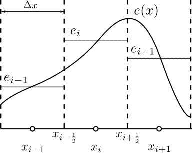
interpolation en espace:
interpolation polynomiale sur chaque cellule
interpolation MUSCL ordre 2 \begin{equation} e(x) = e_i + \sigma_i (x - x_i). \end{equation} pente par différences finies centrées: \begin{equation} \sigma_i = \frac{e_{i+1} - e_{i-1}}{2 \Delta x}. \end{equation}

limiteur MinMod (pour éviter les oscillations)
interpolation d’ordre élevés (schéma ENO, WENO)
schéma DG (Galerkin Discontinu)
# maillage
L=6.0
rho_max=10.
u_max=1.0
# discretisation
nx=201
dx=L/(nx-1)
X  = np.linspace(0,L,nx)
XX = np.zeros(nx+2)
XX[1:-1] = X
XX[0] = -dx
XX[-1]= XX[-2] + dx
def rho_init(rho_feu,XX):
    """ champ initial """
    global rho_max
    rho=rho_feu*(XX/2.0)
    rho=rho*(XX<=2.0).astype(int)
    rho[0]=0.0
    return rho
# condition initiale
rho_s=rho_max
rho0=rho_init(rho_s,XX)
trace(rho0)
def celerite(rho):
    global u_max,rho_max
    return u_max*(1-2*rho/(rho_max))
def Russanov(rho0,cfl,n):
    '''calcul solution avec schéma VF au bout de n iterations'''
    global u_max,rho_max
    rho_n = rho0.copy()
    for i in range(n):
        F = flux(rho_n)
        a = celerite(rho_n)
        # flux et schéma
        Fi = 0.5*(F[:-1]+F[1:]) - \
               0.5*np.maximum(np.abs(a[1:]),np.abs(a[:-1]))*(rho_n[1:]-rho_n[:-1])
        rho_n[1:-1] = rho_n[1:-1] - cfl*(Fi[1:]-Fi[:-1])
        # cdt neumann
        rho_n[0] = rho_n[1]
        rho_n[-1]= rho_n[-2]
    return rho_n.copy()
CFL=0.5
Nit=8
rho_s=rho_max
rho0=rho_init(rho_s,XX)
rho=rho0.copy()
plt.figure(figsize=(12,6))
plt.ylim([0,12])
plt.plot(XX,rho,lw=3,label="it=0")
for it in range(Nit):
    rho=Russanov(rho,CFL,40)
    plt.plot(XX,rho,lw=3,label="it=%d"%it)
plt.legend(loc=0)

passage d’un feu au rouge
Au feu rouge en $x=4$ on a une accumulation de voitures à l’arret avec un flux de voitures arrivant à gauche correspondant à 50% du traffic maximum
la condition initiale:
$$ \rho(x,0) = \left\{ \begin{array}{cc} 0.5 \rho_{\rm max} & 0 \leq x < 3\ \rho_{\rm max} & 3 \leq x \leq 4 \ \end{array} \right. $$# maillage
L=4.0
rho_max=10.
u_max=1.0
# discretisation
nx=201
dx=L/(nx-1)
X = np.linspace(0,L,nx)
XX = np.zeros(nx+2)
XX[1:-1] = X
XX[0] = -dx
XX[-1]= XX[-2] + dx
def rho_init(XX):
    """ champ initial """
    global rho_max
    rho  = 0.5*rho_max*np.ones(XX.size)
    rho += 0.5*rho_max*(XX>=3.0).astype(int)
    return rho
# condition initiale
rho0=rho_init(XX)
a = celerite(rho0)
plt.plot(XX,a)
plt.title('célérité')

CFL=0.5
Nit=8
rho0=rho_init(XX)
rho=rho0.copy()
plt.figure(figsize=(12,6))
plt.ylim([0,12])
plt.plot(XX,rho,lw=3,label="it=0")
for it in range(1,Nit):
    rho=Russanov(rho,CFL,40)
    plt.plot(XX,rho,lw=3,label="it=%d"%it)
plt.legend(loc=0)

perturbation dans un traffic dense
Sur une autoroute de longueur $L$ on a un traffic dense homogène correspondant au maximum du flux.
A l’instant initiale, on a une perturbation (un véhicule ralentis légérement)
def rho_init(rho_s,XX):
    """ champ initial """
    global rho_max
    rho  = rho_s*np.ones(XX.size)
    rho += 0.1*rho_max*np.exp(-(XX-3.)**2/0.04)
    return rho
def simulPerturbation(rho_m):
    ''' perturbation fct densite moyenne rho_m'''
    CFL=0.5
    Nit=7
    # condition initiale
    rho0=rho_init(rho_m,XX)
    rho=rho0.copy()
    plt.figure(figsize=(10,6))
    plt.plot(XX,rho,lw=3,label="it=0")
    for it in range(1,Nit):
        rho=Russanov(rho,CFL,60)
        plt.plot(XX,rho,lw=3,label="it=%d"%it)
    plt.legend(loc=0)
    plt.title("$\\rho_m$ = %f"%(rho_m))
    return
simulPerturbation(rho_m=3)
simulPerturbation(rho_m=8)


interact(simulPerturbation,rho_m=[3,4,5,6,7,8])
expérience
Références
Neville D. Fowkes and John J. Mahony, “An Introduction to Mathematical Modelling,” Wiley & Sons, 1994. Chapter 14: Traffic Flow.
M. J. Lighthill and G. B. Whitham (1955), On kinematic waves. II. Theory of traffic flow and long crowded roads, Proc. Roy. Soc. A, Vol. 229, pp. 317–345. PDF from amath.colorado.edu, checked Oct. 14, 2014. Original source on the Royal Society site.
Practical Numerical Methods with Python: MOOC (Lorena A. Barab, Ian Hawkel, Bernard Kanepen) Numerical MOOC
Fin