Table des matières

1 Discrétisation équation d’Euler
2 Calcul du flux à l’interface
3 Tube à choc de SOD
4 Référence

In [1]:

%matplotlib inline
%autosave 300
import numpy as np
import scipy as sp
import matplotlib.pyplot as plt
from matplotlib import rcParams
rcParams['font.family'] = 'serif'
rcParams['font.size'] = 14
from IPython.core.display import HTML
from IPython.display import display
from matplotlib import animation
css_file = 'style.css'
HTML(open(css_file, "r").read())
# edit metadata   "livereveal": { "scroll": true }
# https://damianavila.github.io/RISE/customize.html

Autosaving every 300 seconds

Out[1]:

Discrétisation équation d’Euler¶

Marc BUFFAT, dpt mécanique, Université Claude Bernard Lyon 1 \begin{equation*} \newcommand{Dx}{\Delta x} \newcommand{Dt}{\Delta t} \newcommand{imh}{{i-\frac{1}{2}}} \newcommand{iph}{{i+\frac{1}{2}}} \newcommand{im}{{i-1}} \newcommand{ip}{{i+1}} \newcommand{dx}[1]{\frac{\partial #1}{\partial x}} \newcommand{dt}[1]{\frac{\partial #1}{\partial t}} \newcommand{gm}{\gamma-1} \newcommand{gmh}{\frac{\gamma-1}{2}} \end{equation*}

Sous forme conservative $$\dt{W} + \dx{F(W)} = 0 $$

$$ W = \left[\begin{array}{c} \rho\ \rho u\ \rho E \end{array}\right] \mbox{ et } F(W) = \left[\begin{array}{c} \rho u\ \rho u^2 +p \ \rho u (E+\frac{p}{\rho}) \end{array}\right] $$

avec $e = \frac{p}{(\gm)\rho},\ E = e +\frac{1}{2} u^2,\ H = E + \frac{p}{\rho}$

matrice jacobienne des fluxs¶

$$ \dx{F(W)} = \mathcal{A} \dx{W} \mbox{ avec } \mathcal{A} = \frac{\partial F}{\partial W}$$

avec

$$ \mathcal{A} = \left[\begin{array}{ccc} 0 & 1 & 0 \ \frac{\gamma -3}{2} u^2 & (3-\gamma)u & \gm \ \gmh u^3 - uH & H - (\gm) u^2 & \gamma u \ \end{array}\right] $$

valeurs propres et vecteurs propres¶

3 valeurs propres

$$\lambda_1 = u - c ,\ \lambda_2=u ,\ \lambda_3= u + c $$

vecteurs propres $$ R_1 = \left[\begin{array}{c} 1 \ u-c \ H-u c \end{array}\right] ,\ R_2 = \left[\begin{array}{c} 1 \ u \ \frac{1}{2} u^2 \end{array}\right] , \ R_3 = \left[\begin{array}{c} 1 \ u+c \ H+u c \end{array}\right] $$

décomposition sur la base des vecteurs propres¶

$$ \Delta W = \alpha_1 R_1 + \alpha_2 R_2 + \alpha_3 R_3 $$

par résolution du système linéaire, on obtiens: $$\alpha_2 = \frac{\gm}{c^2} \left[ \Delta W_1 (H-u^2) + u\Delta W_2 - \Delta W_3 \right]$$ $$\alpha_1 = \frac{1}{2c} \left[ \Delta W_1 (u+c) - \Delta W_2 - c \alpha_2 \right]$$ $$\alpha_3 = \Delta W_1 - (\alpha_1 + \alpha_2)$$

Calcul du flux à l’interface¶

Schéma de Russanov¶

stabilisation du schéma centré avec de la dissipation

fonction de la plus grande (en valeur absolue) des vitesses de propagation
calcul de $s_{max} = \max {|\lambda_k|}$ max des vp de $\mathcal A$
1. maximum des vp à droite et à gauche $$ s_{max} = \max{\left(|vp\ \mathcal{A}(W_i)|, |vp\ \mathcal{A}(W_{i+1})|\right)}$$
2. maximum etat moyen de Roe $$ s_{max} = \max {|vp\ \mathcal{A}(\tilde{W})|}$$
calcul flux $F_\iph$ $$ F_\iph = \frac{1}{2}(F(W_i)+F(W_{i+1})) - \frac{s_{max}}{2} (W_{i+1}-W_i)$$

Schéma de Roe¶

linéarisation du problème de Rieman (schéma Godounov approchée)
calcul d’un état moyen $\tilde{W}$ en $\iph$

\begin{eqnarray} \tilde{u} &=& \frac{\sqrt{\rho_i} u_i + \sqrt{\rho_{i+1}} u_{i+1}}{\sqrt{\rho_i}+\sqrt{\rho_{i+1}}}\ \tilde{H} &=& \frac{\sqrt{\rho_i} H_i + \sqrt{\rho_{i+1}} H_{i+1}}{\sqrt{\rho_i}+\sqrt{\rho_{i+1}}}\ \end{eqnarray}

avec $$\tilde{c}^2 = (\gm)(\tilde{H}-\frac{1}{2} \tilde{u}^2)$$

calcul des valeurs propres $\tilde{\lambda}$ de $\mathcal{A}(\tilde{W})$
calcul des vecteurs propres associés $\tilde{R}_1$,$\tilde{R}_2$,$\tilde{R}_3$
projection de l’écart $\Delta W = W_{i+1} - W_i$ sur ces vecteurs propres: $$W_{i+1} - W_i = \alpha_1 R_1 + \alpha_2 R_2 + \alpha_3 R_3 $$
calcul du flux $F_\iph$

$$ F_\iph = \frac{1}{2} (F(W_{i+1}-F_i) - \frac{1}{2} (\alpha_1 |\lambda_1| R_1 + \alpha_2 |\lambda_2| R_2 + \alpha_3 |\lambda_3| R_3)$$

schéma HLL (Harten, Lax & Van Leer )¶

approximation non linéaire du problème de Rieman (schéma Godounov approchée)
sur l’interface $\iph$ : etat à gauche $i$ et à droite $i+1$
calcul des célérités min à gauche $s_{i}$ et max à droite $s_{i+1}$
à l’aide d’une des 3 approximations:
1. décentré $$ s_i= u_i - c_i ,\ s_{i+1}= u_{i+1} + c_{i+1}$$
2. min et max $$ s_i = \min \left( u_i - c_i, u_{i+1} - c_{i+1}\right), \ s_{i+1} = \max \left( u_i + c_i, u_{i+1} + c_{i+1}\right)$$
3. Roe $$ s_i = \tilde{u} - \tilde{c}, \ s_{i+1} = \tilde{u} + \tilde{c}$$
calcul du flux $F_\iph$
- si $s_i \ge 0 $
$$ F_\iph = F(W_i) $$
- si $s_i \le 0 \le s_{i+1}$
$$ F_\iph =\frac{s_{i+1}F(W_i) - s_i F(W_{i+1}) + s_i s_{i+1}(W_{i+1}-W_i)}{s_{i+1}-s_i} $$
- si $ s_{i+1} \le 0$
$$ F_\iph =F(W_{i+1}) $$

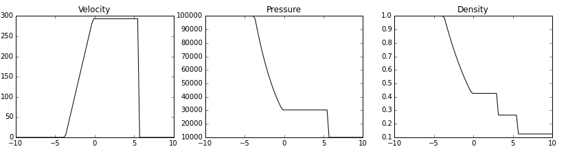
Tube à choc de SOD¶

tube sans dimension $L=1.0$ avec une membrane à $L/2$ $$ \rho_l = 1.0, u_l=0.0, p_l=1.0 \mbox{ et } \rho_r = 0.125, u_r=0.0, p_r=0.1 $$ avec : $$e = \frac{p}{(\gm)\rho},\ E = e +\frac{1}{2} u^2,\ H = E + \frac{p}{\rho}$$

solution à t=0.25

solution SOD

In [2]:

from schemaVF import trace_sol,Russanov,gamma
# parametres
L=1.0
m=1001
X = np.linspace(0,L,m)
dx = L/(m-1)
# maillage fictif (avec cellules fictives)
XX = np.zeros(m+2)
XX[1:-1] = X
XX[0] = -X[1]
XX[-1]= XX[-2]+X[1]
#
CFL = 0.2
tf  = 0.2
N   = int(tf/(CFL*dx))
print("parametres ",CFL,N,m,N*CFL*dx)

parametres  0.2 1000 1001 0.2

In [3]:

# condition initiale
rho_0 = lambda x: (1.0-0.125)*(1-(x>0.5).astype(float))+0.125
pr_0  = lambda x: (1.0-0.1)*(1-(x>0.5).astype(float))  +0.1
W0 = np.zeros((m+2,3))
W0[:,0] = rho_0(XX)
W0[:,2] = pr_0(XX)/(gamma-1)

In [4]:

print("Conditions initiale")
trace_sol(XX,W0)

Conditions initiale

In [5]:

W = Russanov(W0,CFL,N)
trace_sol(XX,W)
print("solution Rusanov a t = ",tf)

solution Rusanov a t =  0.2

Référence¶

Sod, Gary A. (1978), “A survey of several finite difference methods for systems of nonlinear hyperbolic conservation laws,” J. Comput. Phys., Vol. 27, pp. 1–31 DOI: 10.1016/0021-9991(78)90023-2// PDF a partir de HAL
Practical Numerical Methods with Python: MOOC (Lorena A. Barab, Ian Hawkel, Bernard Kanepen) Numerical MOOC

In [ ]:

Cours CFD pour les écoulements compressibles