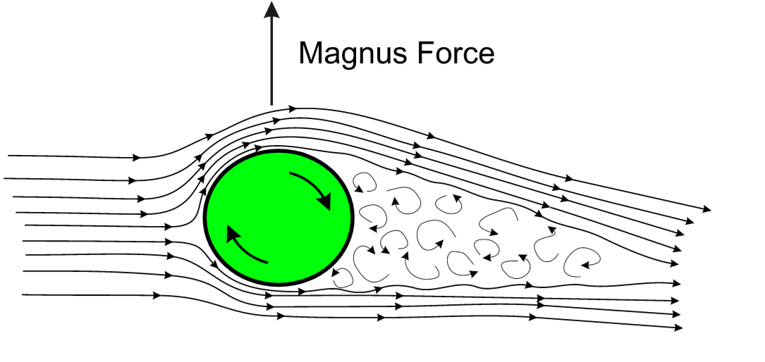
Effet Magnus: écoulement potentiel autour d'un cylindre¶

Marc BUFFAT, département mécanique, université Lyon 1

%matplotlib inline
%autosave 300
import numpy as np
import sympy as sp
import sympy.vector as sv
sp.init_printing()
import matplotlib.pyplot as plt
from matplotlib import rcParams
rcParams['font.family'] = 'serif'
rcParams['font.size'] = 14

Autosaving every 300 seconds

hypothèses¶

fluide parfait,
écoulement incompressible
stationnaire 2D
irrotationel

donc le champ de vitesse découle d'un potentiel

$$\mathbf{U} = \nabla \Phi \mbox{ avec } u = \frac{\partial \phi}{\partial x}, v = \frac{\partial \phi}{\partial y} $$

équation de Laplace pour le potentiel $\Phi$

$$ \Delta \Phi = 0 $$

de même la fonction de courant $$ u = \frac{\partial \psi}{\partial y}, v = -\frac{\partial \psi}{\partial x} $$

vérifie

$$ \Delta \psi = 0 $$

R0 = sv.CoordSys3D('R_0')
display(R0)
x = R0.x
y = R0.y

U0, R, K, Gamma = sp.symbols('U_0 R K Gamma')

Solution potentiel¶

La fonction de courant $\psi$ vérifie

$$\Delta \psi = 0 $$

la solution est obtenue par principe de superposition $$\psi = \psi_1 + \psi_2 + \psi_3$$

# 1/ psi1 correspond à un champ uniforme
psi1 = U0*y

# verification equation de laplace
sv.divergence(sv.gradient(psi1))

# 2/ psi2 correspond à un doublet
psi2 = -K*y/(x**2+y**2)

sv.gradient(psi2)

# verification equation de laplace
sv.divergence(sv.gradient(psi2)).simplify()

# 3/ psi3 correspond à un tourbillon
psi3 = -Gamma/(2*sp.pi)*sp.log(x**2+y**2)

# verification equation de laplace
sv.divergence(sv.gradient(psi3)).simplify()

solution générale¶

$$\psi = \psi_1 + \psi_2 + \psi_3$$

et

$$\Delta \psi = 0$$

psi = psi1 + psi2.subs(K,U0*R**2) + psi3
display(psi)

def trace_solution(psi,R,titre): 
    # conversion fonction numpy
    F = sp.lambdify([R0.x,R0.y],psi,'numpy')
    # grille de calcul
    N = 40
    X1 = np.linspace(-3*R,3*R,N)
    Y1 = np.linspace(-2*R,2*R,N)
    X, Y = np.meshgrid(X1,Y1)
    FXY = F(X,Y)
    # filtrage
    for i in range(N):
        for j in range(N):
            if (X[i,j]**2 + Y[i,j]**2) < 0.8*R**2 : FXY[i,j] = 0.
    # tracer
    plt.figure(figsize=(10,8))
    ax = plt.gca()
    CS = ax.contour(X, Y, FXY, levels=31)
    ax.clabel(CS, inline=1, fontsize=10)
    plt.axis('equal')
    if titre != None : ax.set_title(titre)
    cercle = plt.Circle((0., 0.), R, color='k',zorder=10)
    ax.add_artist(cercle)
    return

cas uniforme $\psi=\psi_1$¶

rayon=1
valnum = { U0:2, R:0, Gamma:0}
psi0 = psi.subs(valnum)
display("psi=",psi0)

'psi='

trace_solution(psi0,rayon,"Ecoulement uniforme")

cas sans rotation $\psi = \psi_1 + \psi_2$¶

valnum = { U0:2, R:rayon, Gamma:0}
psi0 = psi.subs(valnum)
display("psi=",psi0)

'psi='

trace_solution(psi0,rayon,"Cylindre immobile")

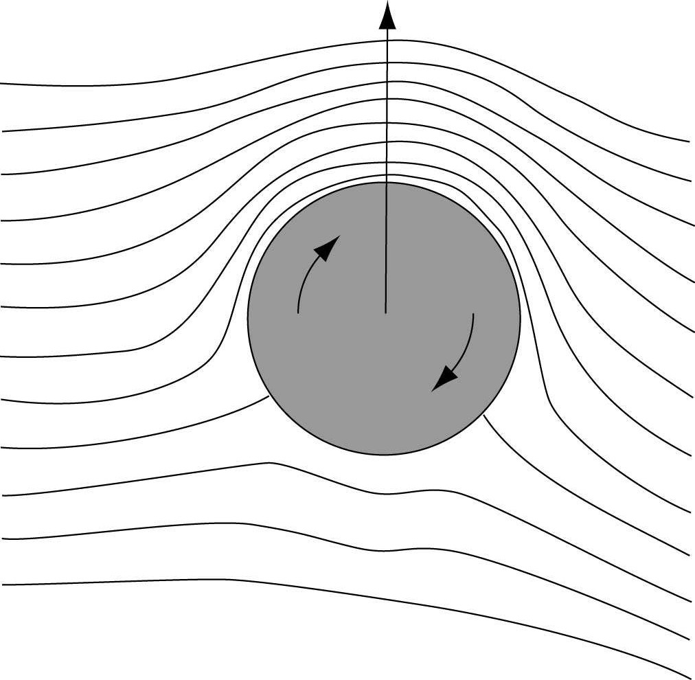
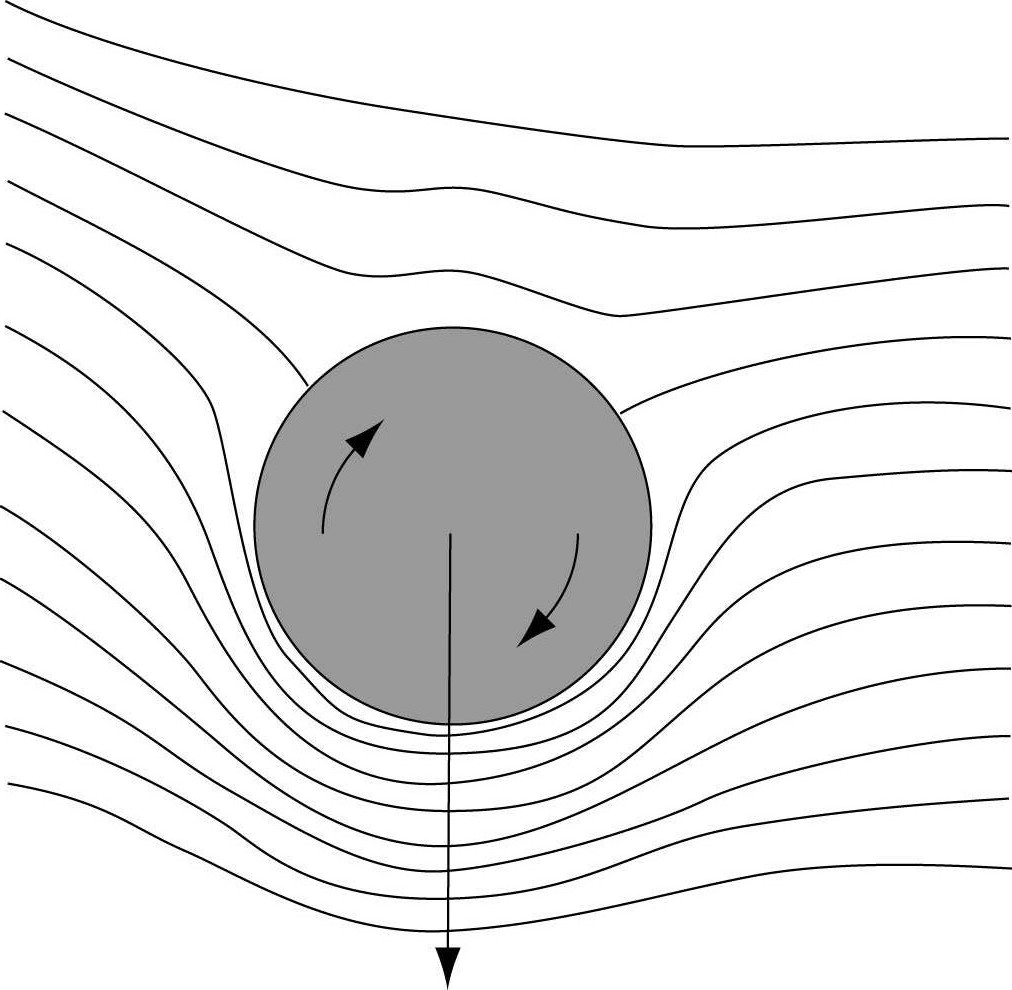
Cas avec rotation: $\psi = \psi_1 + \psi_2 + \psi_3$¶

valnum = { U0:2, R:rayon, Gamma:5}
psi0 = psi.subs(valnum)
display('psi=',psi0)

'psi='

trace_solution(psi0,rayon,"Cylindre en rotation")

Calcul de la pression¶

bilan de qte de mouvement

$$ \frac{\partial \rho \vec{U} } {\partial t} + div(\rho \vec{U} \times \vec{U}) = - \vec{\nabla} p $$ soit en terme d'accélération $$\rho \frac{D \vec{U}}{D t} = \rho \frac{\partial \vec{U} } {\partial t} + \rho \vec{U} . \vec{\nabla} \vec{U} = - \vec{\nabla} p $$

en utilisant la relation vectorielle

$$ \vec{grad}(\frac{1}{2} U^2) = \vec{U} . \vec{grad} \vec{U} + \vec{U} \wedge \vec{rot}\vec{U} $$ on obtiens

$$ \vec{grad}(\frac{\rho}{2} U^2 + p) - \rho \vec{U} \wedge \vec{rot}\vec{U} = \vec{0} $$

ce qui donne Bernoulli si $\vec{rot}\vec{U} = \vec{0}$ $$ \frac{\rho}{2} U^2 + p = cste $$

en notant que $u = \frac{\partial \psi}{\partial y} , v = -\frac{\partial \psi}{\partial x}$ $$ p = \frac{\rho}{2} U_0^2 - \frac{\rho}{2} \vec{\nabla}^2 \psi $$

# demonstration
Nabla = sv.Del()
rho0 = sp.symbols('rho_0')
p = sp.Function('p')(x,y)
u = sp.Function('u')(x,y)
v = sp.Function('v')(x,y)
U = u*R0.i + v*R0.j
display("U=",U)
display("gradU=",Nabla(U))

'U='

'gradU='

# verification de la relation vectorielle
display("1/2grad(U*U)=",sv.gradient(U.dot(U)/2).doit())
display("U.grad(U)=",U.dot(Nabla(U)).doit())
display("U^rot(U)=" ,U.cross(sv.curl(U)))
display("verification (1)-(2)-(3) =",(sv.gradient(U.dot(U)/2).doit() - U.dot(Nabla(U)).doit() - U.cross(sv.curl(U))).simplify())

'1/2grad(U*U)='

'U.grad(U)='

'U^rot(U)='

'verification (1)-(2)-(3) ='

# calcul de la pression
pr = rho0*U0**2/2 -rho0/2*U.dot(U)
display("Pr=",pr)
pr = rho0*U0**2/2-rho0/2*sv.gradient(psi).dot(sv.gradient(psi))
display("Pr=",pr)

'Pr='

'Pr='

valnum = { rho0:1, U0:2, R:rayon, Gamma:0}
pr0 = pr.subs(valnum)
display(pr0)
trace_solution(pr0,rayon,"pression cylindre immobile")

valnum = { rho0:1, U0:2, R:rayon, Gamma:5}
pr0 = pr.subs(valnum)
display(pr0)
trace_solution(pr0,rayon,"pression cylindre en rotation")

Analyse¶

Laquelle de ces 2 configurations est correcte et pourquoi ?

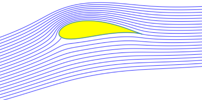
Lien avec la théorie de l'aile¶

transformation conforme dans le plan complexe:

On définit un potentiel complexe $\Phi(z)$: $$\Psi(z) = \phi(x,y) + i \psi(x,y)$$

On définit une transformation conforme $Z=F(z)$ qui préserve les angles dans le plan complexe.

Transformation de Joukovski

$$ Z = z + \frac{C^2}{z} $$

avec $ z = x + i y $ (plan d'origine) et $Z = X + i Y$ (plan transformé)

On obtiens ainsi l'écoulement autour du profil vérifiant la condition de Kutta-Joukovsky au bord de fuite
Equivalence: vitesse de rotation $\omega$ et angle d'incidence $\alpha$
Donc la portance d'un profil d'aile est liée à la circulation de vitesse autour du profil